Cointegration

Cointegration is a statistical method used to test the correlation between two or more non-stationary time series in the long run or for a specified period. The method helps identify long-run parameters or equilibrium for two or more variables. In addition, it helps determine the scenarios wherein two or more stationary time series are cointegrated so that they cannot depart much from the equilibrium in the long run.

• The method determines the sensitivity of two or more variables to the same set of conditions or parameters.
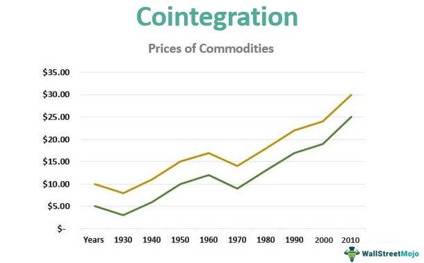
• Let us understand the method with the help of a graph. The prices of two commodities, A and B, are shown on the graph. We can infer that these are perfectly cointegrated commodities in terms of price, as the difference between the prices of both commodities has remained the same for decades. Though this is a hypothetical example, it perfectly explains the cointegration of two non-stationary time series.

• Earlier, linear regression was used as a statistical method to find the relation between two or more time series. However, Granger and Newbold, British economists, argued against linear regression as a technique for analyzing time series for a specified period. As per them, using linear regression sometimes produces false correlations due to the impact of other factors.
• In 1987, Granger and Engle published a paper on this topic. They established the cointegration concept of non-stationary time series to find the correlations. Furthermore, they established that two or more non-stationary time series are cointegrated so that they can move much from equilibrium. The two economists were awarded the Nobel memorial prize in economic sciences for their revolutionary work.

• Cointegration as correlation does not measure whether two or more time-series data or variables move together in the long run. In contrast, it measures whether the difference between their means remains constant or not.
• So, that means that two random variables completely different from each other can have one common trend that combines them in the long run. If this happens, variables are said to be cointegrated.
• Now let’s take the example of Cointegration in pair trading. In pair trading, a trader purchases two cointegrated stocks, stock A at the long position and stock B in the short. The trader was unsure about the price direction for both the stocks but was sure that stock A’s position would be better than that of stock B.
• Now, let us say that if the prices of both the stocks go down, the trader will still make a profit as long as stock A’s position is better than stock B's if both stocks weigh equally at the purchase time.

The three main methods are below:

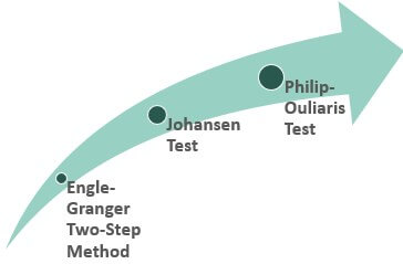
#1 - Engle-Granger Two-Step Method

This method tests the residuals created based on static regression for the presence of unit roots. For example, suppose two non-stationary time series are cointegrated, and the result confirms the stationary characteristic of residuals. However, there are some limitations to this method. For example, suppose there are two or more non-stationary variables. The method will reflect two or more cointegrated relationships. Also, the method is a single equation model. Recent tests like Johansen's and Philip-Ouliaris have addressed some of these limitations.

#2 - Johansen Test

Johansen test is for testing cointegration between several time-series data at a time. This test overcomes the limitation of an incorrect test result for more than two time series of the Engle-Granger method. However, this test is subject to asymptotic properties; i.e., it takes a large sample size because a small sample size would give incorrect or false results. There are two further bifurcations of the Johansen test: the Trace test and the Maximum Eigenvalue test.

#3 - Philip-Ouliaris Test

This test proves that when a residual-based unit root test applies to time series, the cointegrated residuals give asymptotic distribution instead of Dickey-Fuller distribution. The resulting asymptotic distributions are known as Philip-Ouliaris distributions.

The cointegration test is based on the logic that more than two-time series variables have similar deterministic trends that one can combine over time. Therefore, it is necessary for all cointegration testing for non-stationary time series variables. One should integrate them in the same order, or they should have a similar identifiable trend that can define a correlation between them. So, they should not deviate much from the average parameter in the short run. In the long run, they should be reverting to the trend.

This article has been a guide to cointegration and its definition. Here, we discuss history, examples, cointegration methods, and their conditions. You may learn more about financing from the following articles: -

• Econometrics
• Linear Regression in Excel
• Hypothesis Testing
• Positive Correlation
• Net Change Formula