Table Of Contents
Autocorrelation Meaning
Autocorrelation refers to the degree of closeness or correlation between values of the same variable or data series at different periods. This correlation coefficient is also known as lagged or serial correlation.
It is used to identify non-randomness in the presented data. That is, its application involves using it to determine if the data are from a random process or not. Also, the autocorrelation function application will be useful in identifying an apt time series model or a non-linear model with time as the independent variable if the data is not generated from a random process.
Key Takeaways
- Autocorrelation refers to the degree of closeness or correlation between values of the same variable or data series at different periods. It is also known as lagged correlation or serial correlation.
- Generally, its value oscillates between -1 to 1. If the output lies between -1 to 0, then it is a negative correlation, and a positive correlation happens if the output ranges between 0 to 1.
- Traders or analysts use this method to determine the influence of past prices of securities on their future prices.
- In spatial statistics, spatial autocorrelation indicates the systematic spatial variation in a variable. In other words, it determines the connection between nearby observations.
Autocorrelation Explained
The autocorrelation method is applied to the same time series at different time points to determine the relationship between the variable's current and past values. The result of the method discloses whether the different versions of the same time series share a positive or negative correlation. For example, the result can vary from -1 to 1, and if the value is -1 or close to -1, it is a negative correlation; if the value is 1 or close to 1, it is a positive correlation.
Fundamentally, the series data correlates with themselves. The lagged version of the time series is used to determine the degree of correlation between the observations separated by intervals. The correlation can be strong or negative. If the past values do not influence the present values, then the correlation is absent.
It is used in many fields of work. For example, in the financial market, it is applied by stock traders and analysts to understand the degree of similarity, and moving patterns using charts, comprehend the impact of past prices, and predict future prices. Another common example is studying the temperature rise in a weather report. In simple terms, it defines the relationship between a random variable's past and future values. It measures the equation between the observations recorded at different points in time and identifies patterns and trends over the time series.
Autocorrelation Test
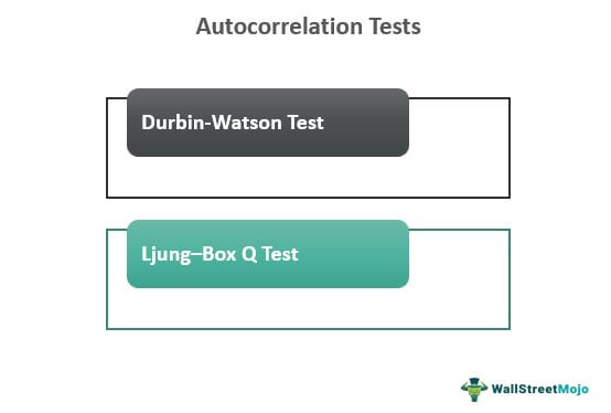
The popularly known tests are:

- Durbin-Watson Test
- Ljung–Box Q Test
Durbin-Watson test
The test gives an output ranging from 0 to 4. The autocorrelation will be
- Closer to 0: Stronger and positive
- Middle: Low
- Closer to 4: Negative
Ljung–Box test
It is also known as the modified Box-Pierce, Ljung–Box Q test, Box test, or Portmanteau test. It tests for the absence of serial autocorrelation for a given lag "k." In addition, it tests for randomness and independence. If the autocorrelations of the residuals are very small, the model is fine; that is, the model does not exhibit a significant lack of fit.
Example
An important example is an analysis of autocorrelation in daily stock returns involving regression analysis using time series data. It gives important implications for market regulation, design of trading mechanisms, and trading strategies that exploit the predictability of stock returns, market efficiency, spread, volatility, trading volume, and liquidity.
Usually, an entry decision at the time of all-time highs is uncommon because lower prices can follow the highest price, that is, the occurrence of a trend reversal. But, at the same time, the emergence of serial autocorrelation displays the tendency of the stock price at the highest level to align within the same direction without a reversal for a reasonable period. So, the active traders can try strategies different from usual, like shifting to an 80/20 portfolio when the scenario is at an all-time high and again choosing a 60/40 portfolio when the price drops.
