Count Characters in Excel

While working with Excel, one often needs to count the number of characters in single or multiple cells. Such characters can be numeric, textual or in the form of a special character. To count characters in excel, the LEN function is used either alone or in combination with other functions of Excel. This function counts alphabets, numbers, spaces, special characters, and punctuation marks.

For example, the formula =LEN(“Let’s set the goals for this year.”) returns 34, which includes 26 alphabets, 6 spaces, 1 apostrophe, and 1 period. The quotes within which the text string is enclosed are excluded from the count.

The purpose of counting characters in excel is to ensure that the length of the string does not exceed the word count limitations set for certain worksheets. Moreover, a character count is essential before releasing a brochure, advertisement, business card or Excel report.

Let us consider a few examples to understand the technique of counting characters in Excel.

Example #1–Count all Characters in Each Cell of a Column

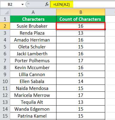
The succeeding image shows some names in column A. We want to count the number of characters in each cell of the range A2:A15. Use the LEN function of Excel.

The steps to count characters in excel by using the LEN function are listed as follows:

Step 1: Enter the following formula in cell B2.

“=LEN(A2)”

Step 2: Press the “Enter” key. Next, drag the fill handle (bottom-right corner) of cell B2 till cell B15. The formula (of cell B2) and the outputs are shown in the succeeding image.

Hence, the total characters in each cell of column A have been counted and returned in the corresponding cell of column B.

Explanation: Apart from the characters of each name, the count (in column B) includes three spaces. One space is between the first and the last name. The remaining two spaces have been deliberately inserted after the last name in each cell.

Hence, to know only the number of letters of a cell (of column A), one needs to subtract 3 from the respective output (of column B).

Note 1: The syntax of the LEN function is “LEN(text).” The “text” is the string whose characters are to be counted. It is a required argument. This argument can either be supplied as a text string within double quotes or as a reference to a cell containing text.

The argument “text” does not mean that the cell should necessarily contain a text string. The LEN function can count any kind of character contained by a cell.

Note 2: The LEN function counts all kinds of spaces, whether leading, trailing, or between the text strings.

Example #2–Count the Characters Left in a Cell After Excluding a Specific Character

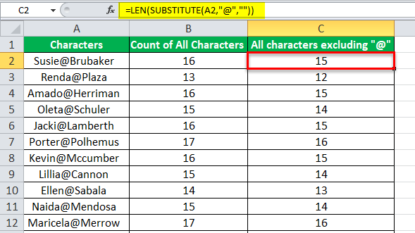
Working on the dataset of example #1, we have placed the character “@” between the first and the last names. Count the number of characters in each excel cell of the range A2:A12. The count should exclude the character “@.”

Use the LEN and SUBSTITUTE functions of excel.

The steps to count the number of characters by using the given excel functions are listed as follows:

Step 1: Enter the following formula in cell C2.

“=LEN(SUBSTITUTE(A2,“@”,“”))”

Step 2: Press the “Enter” key. Then, drag the fill handle of cell C2 till cell C12. The formula (of step 1) and the outputs are shown in the following image.

Hence, the length of the string excluding character “@” has been obtained in column C.

Explanation: In the given formula (entered in step 1), the SUBSTITUTE function is processed first, followed by the LEN function. This formula works as follows:

• The SUBSTITUTE function replaces the character “@” with an empty string. An empty string is represented by a pair of double quotation marks (like “”).
• Next, the LEN function realizes that the character “@” has been excluded from each cell of column A. Consequently, it counts the characters left after such exclusion.

Notice that each output of column C is one less than the corresponding output of column B. This is because, in column B, the LEN function has counted a space between the first and the last names (refer to the “explanation” of example #1). This space has been replaced by the character “@” in the current example. Further, this single character is excluded from the count.

Note 1: The syntax of the SUBSTITUTE function is shown in the following image.

The “text” argument is the text string (or the reference to a cell containing text) in which characters need to be substituted. The “old_text” is the text to be replaced. The “new_text” is the text with which replacement has to be carried out. The “instance_num,” being an optional argument, indicates which occurrence of the “old_text” should be replaced by the “new_text.”

Note 2: In the current example, the reference “A2” is the “text” argument of the SUBSTITUTE function. The “old_text” argument is “@” and the “new_text” argument is an empty string (“”). Since the “instance_num” argument has been omitted, every occurrence of the “old_text” has been replaced with “new_text.”

At present, there is only one occurrence of “@” in each name (of column A). Had there been multiple occurrences of this character in a single name, all instances would have been excluded from the count by the LEN function (as “instance_num” is omitted).

Note 3: The SUBSTITUTE function can be used with numbers too. However, remember that the SUBSTITUTE is a case-sensitive function. This means that “A” and “a” are treated differently. For more details related to the SUBSTITUTE function, click the hyperlink given in the explanation of this example.

Example #3–Count the Occurrence of a Specific Character in a Cell

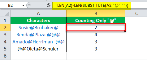
Working on the dataset of example #1, we have inserted character “@” multiple times in four names of column A. Count the number of occurrences of this character in each cell of the range A2:A5.

Use the LEN and SUBSTITUTE functions of Excel.

The steps to count the number of occurrences of the given character are listed as follows:

Step 1: Enter the following formula in cell B2.

“=LEN(A2)-LEN(SUBSTITUTE(A2,“@”,“”))”

Step 2: Press the “Enter” key. Next, drag the formula of cell B2 till cell B5. The formula (of step 1) and the outputs are shown in the following image.

Hence, the number of occurrences of character “@” (in each cell of column A) has been obtained in column B.

Explanation: In the given formula (entered in step 1), we have subtracted the count of characters excluding “@” from the total length of the string.

The count excluding “@” is assessed by the formula “LEN(SUBSTITUTE(A2,“@”,“”).” The count of the entire string is computed by the formula “LEN(A2).” So, when the former is subtracted from the latter, we obtain the count of the character “@.”

Hence, in cell A2, the character “@” appears twice. Likewise, in cell A3, this character appears four times. Irrespective of the placement of this character, it has been counted by the LEN and SUBSTITUTE formula.

Note: For the syntax of the SUBSTITUTE formula, refer to “note 1” given at the end of example #2.

Example #4–Count all Characters of a Vertical Range

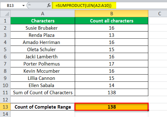
Working on the dataset of example #1, we want to sum the characters of the entire range A2:A10. Use the SUMPRODUCT and LEN functions of Excel.

The steps to count the characters of the entire excel range (A2:A10) are listed as follows:

Step 1: Enter the following formula in cell B13.

“=SUMPRODUCT(LEN(A2:A10))”

Step 2: Press the “Enter” key. The formula and the resulting output are shown in the following image.

Hence, the sum of characters of the entire range (A2:A10) is 138.

Explanation: The LEN function alone cannot handle arrays. So, we have enclosed the LEN within the SUMPRODUCT (in step 1) to sum the characters of the entire range (A2:A10).

The formula, entered in step 1, works as follows:

• The LEN function counts the number of characters in each cell of the range A2:A10. This count is returned by the function as an array of numbers.
• The SUMPRODUCT sums the array returned by the LEN function. So, the array of 9 numbers {16,13,16,15,16,17,16,15,14} is summed up by the SUMPRODUCT function.

Notice that the two trailing spaces (after each name) in each cell of the given range have also been counted by the LEN function.

To cross-check the final output returned by the LEN and SUMPRODUCT formula (entered in step 1), one can add the individual outputs given in the range B2:B10. The sum of values of the range B2:B10 is 138.

Note 1: The syntax of the SUMPRODUCT function is shown in the following image.

The arguments “array1,” “array2,” “array3,” etc., are the arrays whose values need to be multiplied and then added. “Array1” is required, while the remaining “array” arguments are optional. When a single array is specified, the SUMPRODUCT returns the sum of the values of that array.

Note 2: Alternatively, one can sum the characters of the range A2:A10 by using the formula “=SUM(LEN(A2:A10)).” Enter this formula without the beginning and ending double quotation marks. Once entered, press the keys “Ctrl+Shift+Enter” together.