What Are Errors In Excel?
Errors in Excel is common. They occur when there are mistakes in the functions and formulas. MS Excel is popular for only its most useful automatic calculation feature, which we achieve by applying various functions and formulas. But while using formulas in Excel cell, we get multiple types of errors.
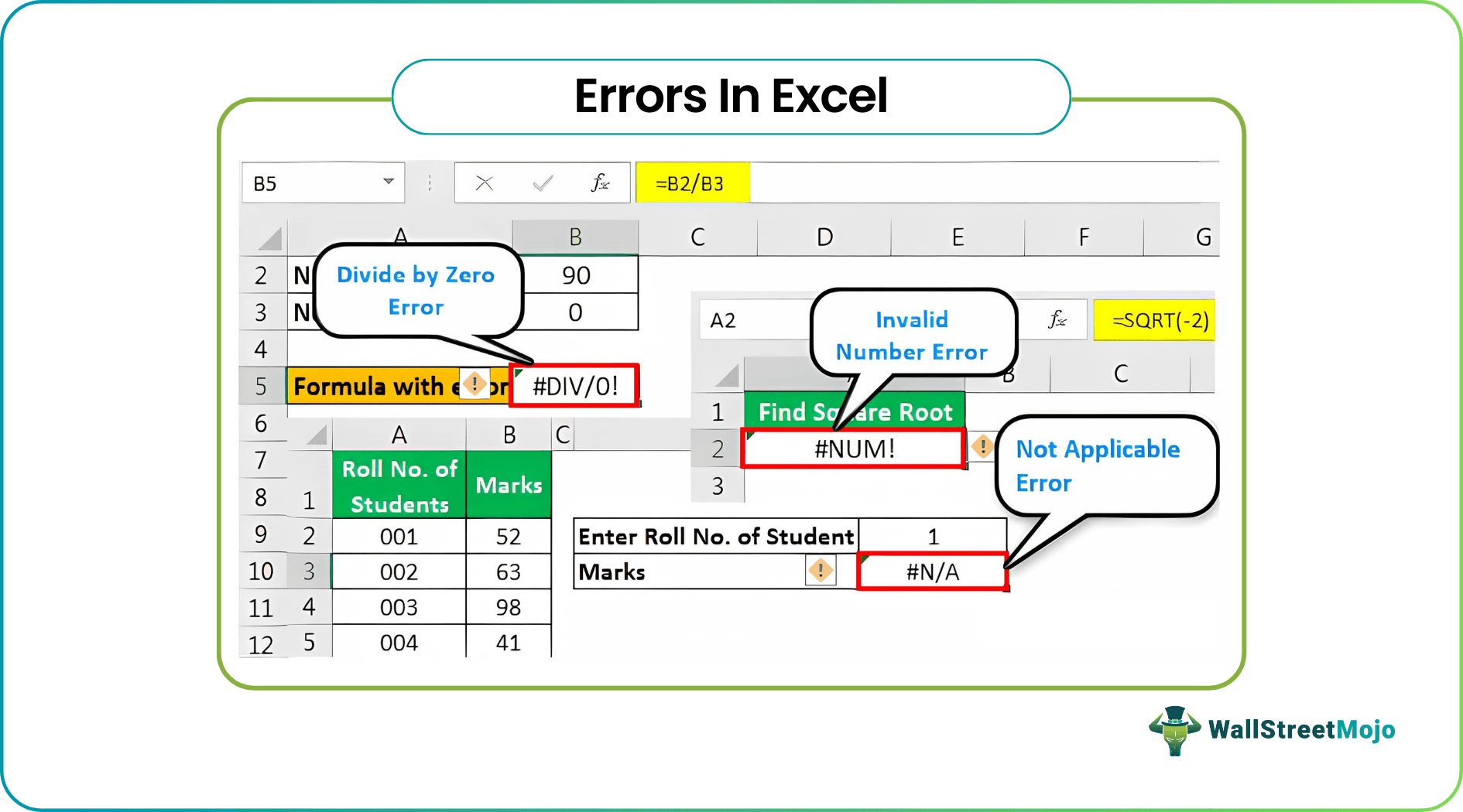
The error can be:
- #DIV/0
- #N/A
- #NAME?
- #NULL!
- #NUM!
- #REF!
- #VALUE!
- #####
- Circular Reference
Key Takeaways
- Errors in Excel are possible while utilizing the formulas in Excel cells. However, Excel provides an automatic calculation. It is an Excel feature that makes it an in-demand choice.
- The list of common Excel errors are #DIV/0, #N/A, #NAME, #NULL!, #NUM!, #REF!, #VALUE! and circular reference.
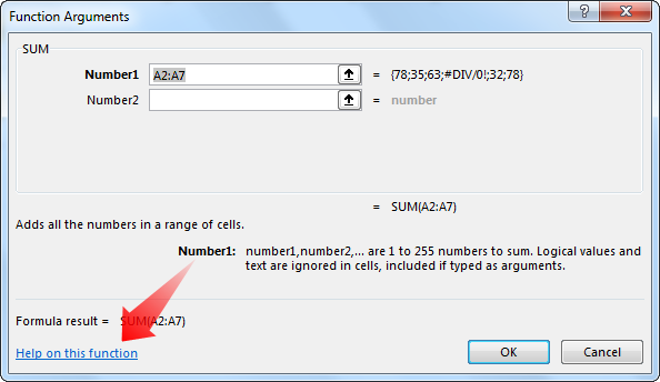
- To fix the formula errors in Excel, one must click on the “Insert Function” under the “Formulas” tab and choose “Help on this function.”
- To avert the #NAME? Error, select the desired function from the drop-down Excel list when typing the “=” sign—press “Tab” to select.
List Of Top 10 Errors In Excel
Let us learn the meaning of top 10 errors and how to fix them in Excel with detailed examples.
1 – #DIV/0 Error
#DIV/0! Error is received when we work with a spreadsheet formula, which divides two values in a formula and the divisor (the number being divided by) is zero. It stands for divide by zero error.
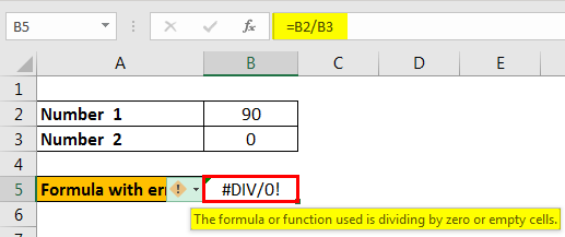
Here, in the above image, we see that number 90 is divided by 0. That is why we get the #DIV/0! Error.
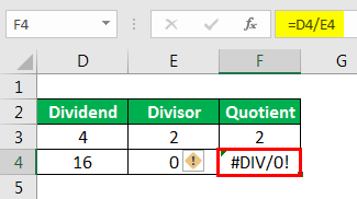
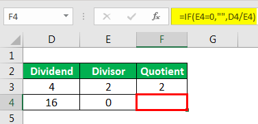
The first and foremost solution is to divide only with cells with a value not equal to zero. But there are situations when we also have empty cells in a spreadsheet. In that case, we can use the IF function as below.
Follow the steps below to use the IF function to avoid the #DIV/0! Error.
- Suppose we are getting a #DIV/0! Error as follows:

- To avoid this error, we can use the IF function as follows:

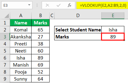
2 – #N/A Error
This error means “no value available” or “not available.” It indicates that the formula cannot find the value that we suppose it may return.
For example, using Excel’s VLOOKUP, HLOOKUP, MATCH, and LOOKUP functions, we may get this error if we do not find referenced value in the source data as an argument.
- When the source data and the lookup value are not of the same data type:
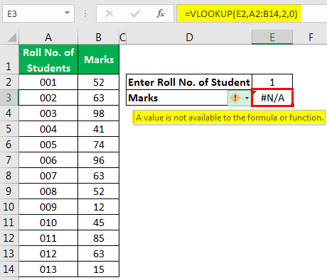
In the above example, we have entered “Roll No. of Students” as a number, but the roll numbers of students are stored as text in the source data. That is why the #N/A error appears.
To resolve this error, we can either enter the roll number as text-only or use the TEXT formula in Excel in the VLOOKUP function.
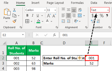
Solution 1: To Enter The Roll Numbers As Text
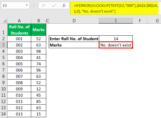
Solution 2: Use The TEXT Function
We can use the TEXT function in the VLOOKUP function for the lookup_value argument to convert entered numbers to TEXT.

We could also use the IFERROR function in Excel to display the message if VLOOKUP cannot find the referenced value in the source data.
3 – #NAME? Error
This error is displayed when we usually misspell the function name.
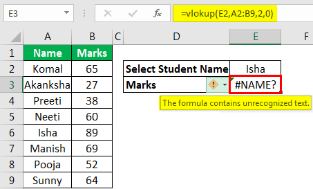
We can see in the above image that VLOOKUP is not spelled correctly; that is why #NAME? Error is being displayed.
To resolve the error, we need to correct the spelling.
4 – #NULL! Error
This error is usually displayed when cell references are not specified correctly.
We get this error when we do not use the space character appropriately. The space character is called the “intersect operator,” which specifies the range that intersects each other at any cell.
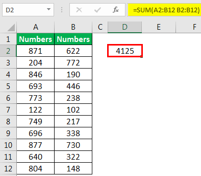
In the below image, we have used the space character, but the ranges A2:A12 and B2:B12 are not intersecting; that is why this error is displayed.

In the below image, we can see that the sum of range B2:B12 is being displayed in cell D2 as while specifying a range for SUM function, we have picked up two references (with space character), which overlap each other for range B2:B12. That is why the sum of the B2:B12 range is displayed.
#NULL! an error can also be displayed when we use intersect operator (space character) instead of:
- Mathematical Operator (Plus Sign) to sum.
- Range Operator (Colon Sign) to specify the start and end cell for a range.
- Union Operator (Comma Sign) to separate individual cell references.
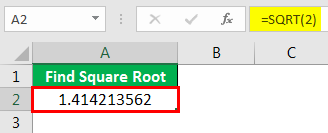
5 – #NUM! Error
This error is usually displayed when a number for any function argument is found invalid.
Example 1
To find out the square root in Excel of a negative number is not possible as the square of a number always has to be positive.
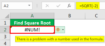
To solve the error, we need to make the number positive.
Example 2
MS Excel has a range of numbers that we can use. The number smaller than the shortest number or number greater than the longest number due to the function can return an error.
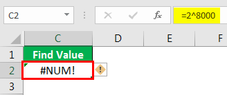
Here, we can see that we have written the formula as 2^8000, which yields results greater than the longest number; that is why #NUM! Error is being displayed.
6 – #REF! Error
This error stands for reference error. This error usually comes when
- We accidentally deleted the cell which we referenced in the formula.
- We cut and paste the referenced cell in different locations.
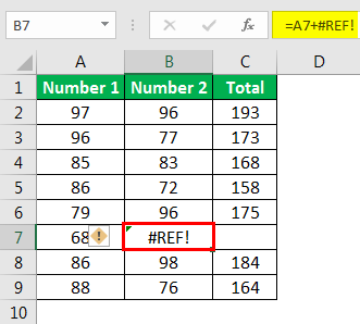
As we deleted cell B7, then cell C7 shifted left to take the place of B7, and we got a reference error in the formula as we deleted one of the referenced cells of the formula.
7 – #VALUE! Error
This error comes when we use the wrong data type for a function or formula. For example, we can add only numbers. But if we use any other data type like text, this error will be displayed.

8 – ###### Error
This error is displayed when the column width in Excel is not enough to show the stored value in the cell.
Example
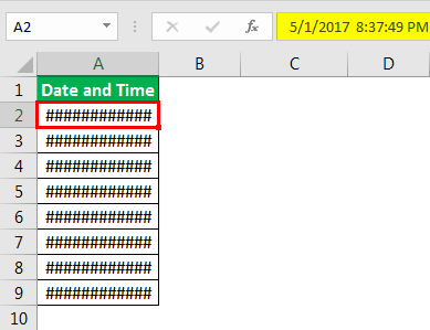
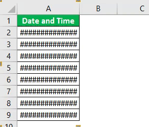
In the below image, dates and times are written in the cells. But, as column width is not enough, ##### is being displayed.
To resolve the error, we need to increase the column width as per requirement using the “Column Width” command available in the “Format” menu in the “Cell Size” group under the “Home” tab, or we can double click on the right border of the column.
9 – Circular Reference Error
This type of error comes when we reference the same cell in which we are writing the function or formula.
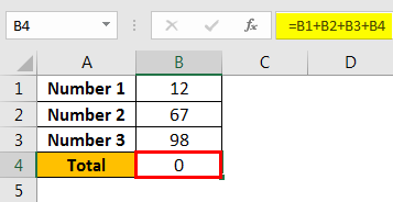
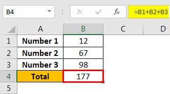
The above image shows that we have a sum of 0 as we have referenced B4 in the B4 cell itself for calculation.
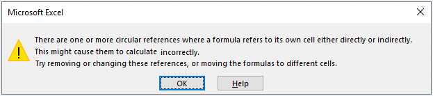
Whenever we create this type of circular reference in Excel, Excel alerts us about the same too.
To resolve the error, we need to remove the reference for the B4 cell.
Function To Deal With Excel Errors
We have various functions to deal with these errors.
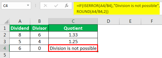
1 – ISERROR Function
This function is used to check whether there would be an error after applying the function or not.
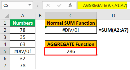
2 – AGGREGATE Function
This function ignores error values. Therefore, when we know that there can be an error in the source data, we need to use this function instead of the SUM, COUNT function, etc.
Example
We can see that the AGGREGATE function avoids error values.
Important Things To Note
- To resolve any error in the formula, we can take online help also. First, we need to click on the “Insert Function” button under the “Formulas” tab and choose “Help on this function.”
- To avoid the #NAME? Error, we can choose the desired function from the drop-down list opened when we start typing any function in the cell, followed by the “=” sign. Next, we need to press the “Tab” button on the keyboard to select a function.
Frequently Asked Questions (FAQs)
1. How to ignore all errors in Excel?
To ignore all errors in Excel, one can turn off the background error-checking feature. One must follow the following steps:
1. Go to the Excel ribbon and choose the “File” tab.
2. Then, from the dropdown menu, select “Options.”
3. After that, in the “Excel Options” dialog box, one can choose the “Formulas” tab.
4. Then, locate the “Enable background error checking” checkbox and unchoose it.
5. Lastly, click on “OK.”
2. What is the shortcut for ignore all errors in Excel?
To remove in-cell error warnings from a selected range of cells, a quick and easy way is to press the keyboard shortcut Alt+Menu Key+I. This command clears the warnings, represented as small green triangles at the top-left corner, from the selected cells with speed and efficiency.
3. How to get rid of a #VALUE error in Excel with IF statement?
There are several complexities involved in building IF statements. It is standard to receive the #VALUE! Error. However, one can protect the error by considering the error-handling functions like ISERROR, ISERR, or IFERROR in the Excel formula.
Recommended Articles
This article is a guide to Errors in Excel. Here, we discuss the top types of errors in Excel and functions to deal with them with the help of examples. You can learn more about Excel from the following articles: –