Part of our LOOKUP Functions in Excel guide
What is LOOKUP Excel Function?
The LOOKUP excel function searches a value in a range (single row or single column) and returns a corresponding match from the same position of another range (single row or single column). The corresponding match is a piece of information associated with the value being searched.
For example, the branch code (search value) can be used to retrieve the profits of different bank branches (corresponding match). Being a lookup and reference function, the LOOKUP has two varieties–vector and array.
The VLOOKUP and HLOOKUP are improved versions of the LOOKUP function.
The LOOKUP is different from the VLOOKUP function in the sense that the former looks for a match in a one-row or one-column range while the latter searches the entire data table.
LOOKUP Excel Function–Syntax 1 (Vector Form)
In the present context, a one-row or one-column range is known as a vector. In this form, the function searches a particular value in one vector and returns a corresponding value at the same position from another vector.
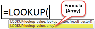
The syntax of the vector form is shown in the following image:

The function accepts the following arguments in the vector form:
- Lookup_value: This is the value to be searched.
- Lookup_vector: This is the one-row or one-column range in which the value is to be searched. It should be sorted in alphabetical order or ascending order to obtain correct results.
- Result_vector: This is the one-row or one-column range from which the output is to be returned. The output returned is in the same position as the “lookup_value.”
The “lookup_value” and “lookup_vector” are mandatory arguments while “result_vector” is optional.
Note: The “lookup_vector” and the “result_vector” both are one-row or one-column range with the same size. If the latter is omitted, Excel returns a value from the former.
LOOKUP Excel Function Explained in Video

LOOKUP Excel Function–Syntax 2 (Array Form)
In this form, the function searches a specified value in the first row or column of the array and returns a corresponding value at the same position from the last row or column of the array.
The syntax of the array form is shown in the following image:
The function accepts the following mandatory arguments in the array form:
- Lookup_value: This is the value to be searched.
- Array: This is the array or range where the value is to be searched.
The first row or column of the array is similar to the “lookup_vector” (vector form). The last row or column of the array is similar to the “result_vector” (vector form).
The Explanation of the LOOKUP Function
The LOOKUP function works on a close match or an approximate match. The two forms of the function are explained in the current section.
The Vector Form
The LOOKUP function looks for the exact “lookup_value” in the “lookup_vector” and returns the output at the same position from the “result_vector.” The possibilities are stated as follows:
- If the function does not find an exact match, it looks up the largest value in the “lookup_vector,” which is less than or equal to the “lookup_value.”
- If the “lookup_value” is smaller than all the values of the “lookup_vector,” the function returns “#N/A error”.
- If the “lookup_value” is greater than all the values of the “lookup_vector,” the function matches with the last value of the array.
- If the “lookup_value” occurs multiple times in the “lookup_vector,” the function considers the last occurrence of the former.
The “lookup_value,” “lookup_vector,” and “result_vector” can be a number, text string, date, currency, and so on.
The Array Form
The LOOKUP function searches for a value according to the dimensions (size) of the array. The possibilities are stated as follows:
- If the number of rows is more than the columns (column size is greater than or equal to the row size), the function searches for the “lookup_value” in the first column.
- If the number of columns is more than the rows (row size is greater than the column size), the function searches for the “lookup_value” in the first row.
How to use the LOOKUP Function in Excel?
Let us understand the working of the LOOKUP function with the help of examples.
Example #1–Vector Form
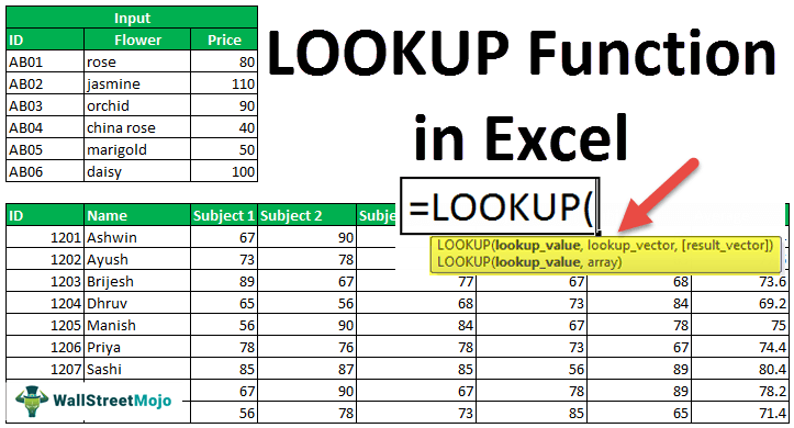
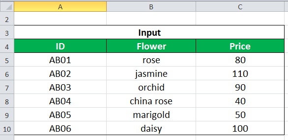
The succeeding table shows a list of flowers, the identifier (ID), and the current price. The output to be retrieved with the help of the LOOKUP function is stated as follows:
a. The price of the flower given its ID
b. The price of the flower given its name
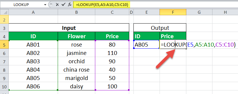
a. We use the following syntax for extracting the price of the flower with its ID.
“=LOOKUP(ID_to_search,A5:A10,C5:C10)”
Since the value to be searched can be supplied as a cell reference, enter E5 in the formula. This is shown in the succeeding image.
“=LOOKUP(E5,A5:A10,C5:C10)”
The formula returns 50.
b. We use the following formula for extracting the price of the flower with its name.
“=LOOKUP(“orchid”,B5:B10,C5:C10)”
The formula returns 90.
Example #2–Vector Form
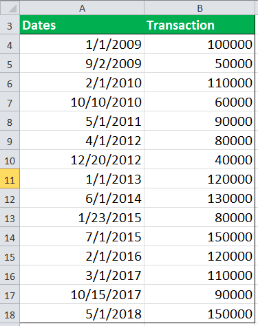
The following table displays the transaction costs (in dollars) incurred on various dates beginning from January 2009. The output to be retrieved with the help of the LOOKUP function is stated as follows:
a. The cost of the last transaction of 2012
b. The cost of the last transaction of March
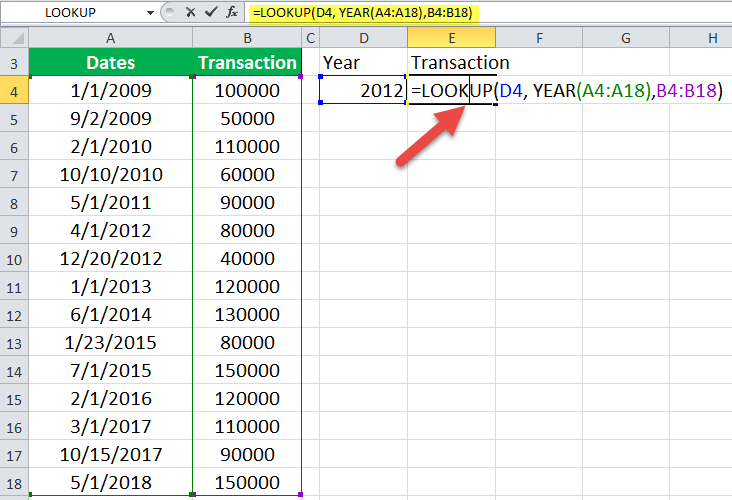
a. We use the following formula for extracting information on the last transaction of 2012.
“=LOOKUP(D4,YEAR(A4:A18),B4:B18)”
The “YEAR(A4:A18)” retrieves the year from the dates given in A4:A18. Since D4=2012, the formula returns $40000.
b. We use the following formula for extracting the cost of the last transaction of March.
“=LOOKUP(3,MONTH(A4:A18),B4:B18)”
The “MONTH(A4:A18)” extracts the month from the dates given in A4:A18. The formula returns $110000.
Example #3–Vector Form
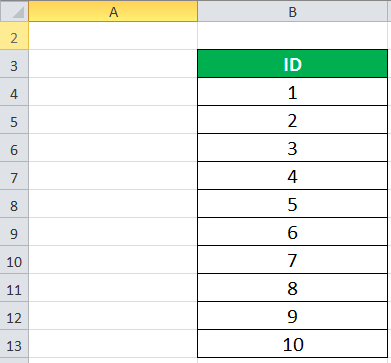
The following table shows a list of IDs in column B. We want to retrieve the last entry of the column with the help of the LOOKUP function. The situations for retrieval are stated as follows:
a. When IDs are listed from 1 to 10
b. When IDs are listed from 1 to 20
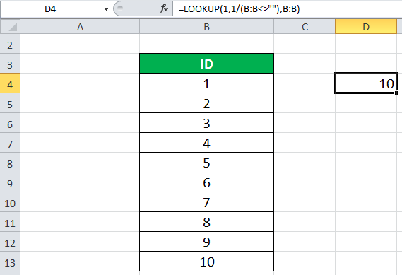
a. We use the following formula to extract the last entry of column B.
“=LOOKUP(1,1/(B:B<>””),B:B)”
In the formula, the “lookup_value” is 1, the “lookup_vector” is 1/(B:B<>””), and the “result_vector” is B:B.
The (B:B<>””) forms an array of “true” and “false” where the former means a value is present, while the latter means it is absent. This array is divided by 1 to form another array of “1” and “0” which corresponds to “true” and “false” respectively.
Since the “lookup_value” is 1, the LOOKUP function looks for 1 in the array of “1” and “0.” It matches the “lookup_value” with the last “1” and returns a corresponding match. In this case, the corresponding match is the actual “lookup_value” at the same position, which is 10.
The output of the formula is 10, as shown in the following image.
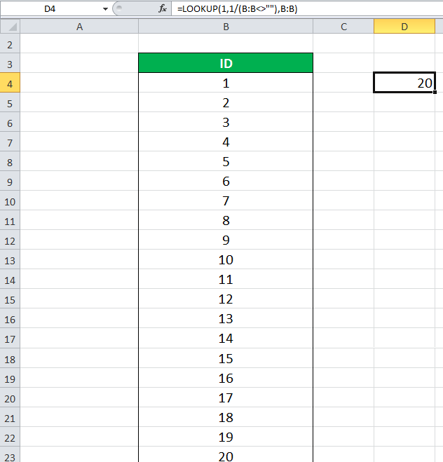
b. We use the same formula (explained in the preceding section) to extract the last entry of column B.
“=LOOKUP(1,1/(B:B<>””),B:B)”
The formula returns 20, as shown in the following image.
Example #4–Array Form
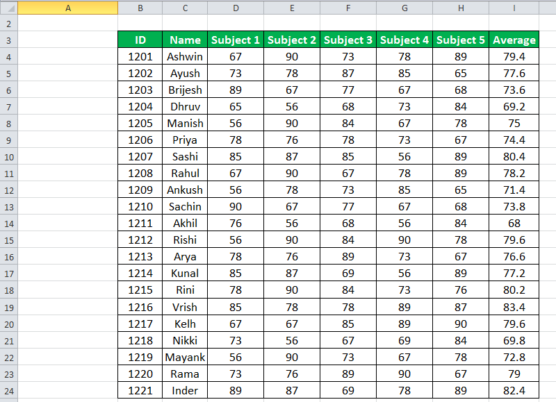
The following table (B3:I24) shows the roll numbers (ID), names of the students, marks in five subjects, and average marks. We want to retrieve the average marks with the help of the student ID.
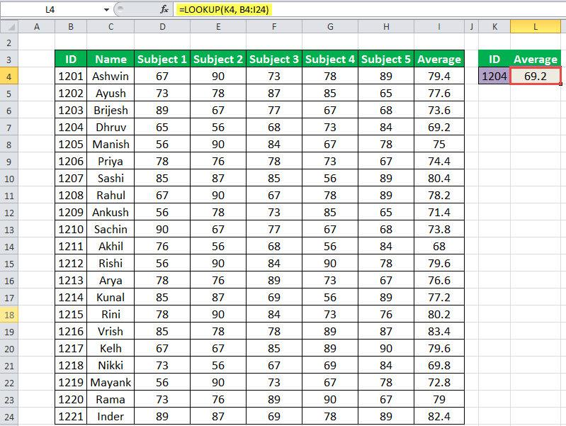
Since the ID to look for is in cell K4, the following formula is used.
“=LOOKUP(K4,B4:I24)”
The formula returns the corresponding average marks of the student Dhruv (ID 1204). The output is 69.2, as shown in the following image.
Applications
The function is used in the following situations:
- To extract the price of an item using its identifier
- To find the location of a book in the library
- To obtain the last transaction cost for a given month or year
- To check the latest price of a product
- To find the last row within a range of numerical or textual data
- To retrieve the last transaction date
Note: The LOOKUP function of Excel is not case-sensitive implying that it treats the uppercase and lowercase letters the same.
Frequently Asked Questions (FAQs)
Define the LOOKUP function of Excel.
The LOOKUP function looks for a value in a single row or column and returns a corresponding value having the same position from another row or column. The look up and the extraction data both should be a one-row or a one-column range.
The LOOKUP function of Excel has two forms which are explained as follows:
• Vector form–The “lookup_value” is searched in the “lookup_vector” and a corresponding match is returned from the “result_vector.” The syntax is stated as follows:
“LOOKUP(lookup_value,lookup_vector,)”
The first two arguments are mandatory and the last one is optional.
• Array form–The “lookup_value” is searched in the first row or column of the “array” and a corresponding match is returned from the last row or column of the “array.” The syntax is stated as follows:
“LOOKUP(lookup_value,array)”
Both the arguments are mandatory.
When should the LOOKUP function of Excel be used?
The usage of the general LOOKUP function, the vector, and the array forms is mentioned as follows:
• The general function is used when there is a need to retrieve an associated piece of information from a one-row or a one-column range.
• The vector form is used when there is a need to specify the range from which a corresponding match is to be returned.
• The array form is used when the lookup or search value is in the first row or column and the corresponding match is in the last row or column.
Note: It is recommended to use the VLOOKUP and HLOOKUP as an alternative to the array form.
What is the difference between the LOOKUP, VLOOKUP, and HLOOKUP functions of Excel?
The differences between the three functions are stated as follows:
• The LOOKUP searches for a value in a one-row or one-column range. In contrast, the VLOOKUP and HLOOKUP search for a value in two or more columns or rows respectively.
• The array form of the LOOKUP searches the “lookup_value” according to the dimensions of the array. In comparison, the VLOOKUP and the HLOOKUP search for the “lookup_value” in the first column and the first row respectively.
• The LOOKUP looks for an approximate match while the VLOOKUP and HLOOKUP work for both approximate and exact matches.
• The LOOKUP has cross functionality implying that it is capable of performing both vertical and horizontal lookups. On the other hand, the VLOOKUP and HLOOKUP are limited to only vertical and horizontal lookups respectively.
Recommended Articles
For more on LOOKUP Functions in Excel, explore these related articles from our LOOKUP Functions in Excel guide.