MATCH Function in Excel
The MATCH function looks for a specific value and returns its relative position in a given range of cells. The output is the first position found for the given value. Being a lookup and reference function, it works for both an exact and approximate match. For example, if the range A11:A15 consists of the numbers 2, 9, 8, 14, 32, the formula “MATCH(8,A11:A15,0)” returns 3. This is because the number 8 is at the third position.
In simple words, the MATCH formula is given as follows:
“MATCH(value to be searched, array, exact or approximate match [1, 0 or -1])”
The Syntax of the MATCH Excel Function
The syntax of the function is shown in the following image:

The function accepts the following arguments:
- Lookup_value: This is the value to be searched in the “lookup_array.”
- Lookup_array: This is the array or range of cells where the “lookup_value” is to be searched.
- Match_type: This takes the values 1, 0, or -1 depending on the type of match.
For instance, you may want to search a specific word (lookup_value) in the dictionary (lookup_array).
The arguments “lookup_value” and “lookup_array” are mandatory, while “match_type” is optional.
The Values of “Match_Type”
The “match_type” can take any of the following values:
Positive one (1): The function looks for the largest value in the “lookup_array,” which is less than or equal to the “lookup_value.” The data is arranged in alphabetical (A to Z) or ascending order and an approximate match is returned.
Zero (0): The function looks for an exact match of the “lookup_value” in the “lookup_array.” The data is not required to be arranged.
Negative one (-1): The function looks for the smallest value in the “lookup_array,” which is greater than or equal to the “lookup_value.” The data is arranged in reverse order of alphabets (Z to A) or descending order and an approximate match is returned.
Note: The default value of “match_type” is 1.
How to use the MATCH Function in Excel? (With Examples)
Let us understand the working of the MATCH formula with the help of examples.
Example #1–Exact Match
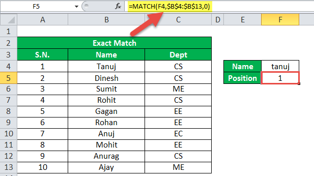
The succeeding table shows the serial number (S.N.), name, and department of ten employees in an organization. We want to find the position of the employee “Tanuj.”
We apply the following formula.
“=MATCH(F4,$B$4:$B$13,0)”
The “match_type” is set at 0 to return the exact position of “Tanuj” (lookup_value) from the range $B$4:$B$13 (lookup_array). The output is 1.
Example #2–Approximate Match
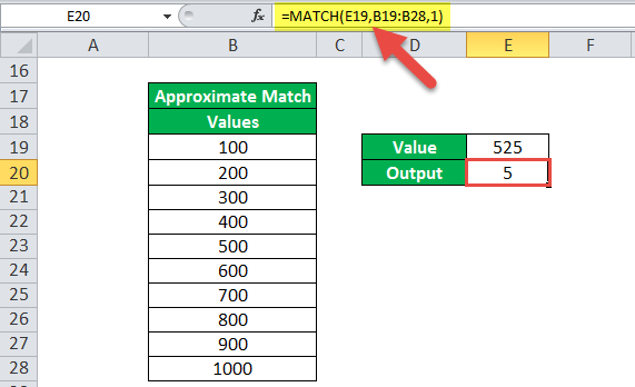
The succeeding list shows the values from 100 to 1000. We want to find the approximate position of the value 525.
We apply the following formula.
“=MATCH(E19,B19:B28,1)”
The “match_type” is set at 1 to return the approximate match of 525 (lookup_value) from the range B19:B28 (lookup_array).
The MATCH function looks for the largest value (500), which is less than 525 in the given array. Hence, the output is 5.
Example #3–Wildcard Character (Partial Match)
The MATCH function supports the usage of wildcard characters (? and *) in the “lookup_value” argument. Let us consider an example of the same.
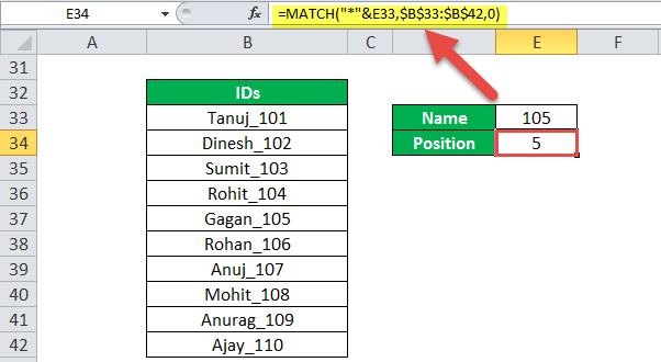
The succeeding list shows ten IDs of the various employees of an organization. We want to find the position of the ID ending with 105.
We apply the following formula.
“=MATCH(“*”&E33,$B$33:$B$42,0)”
The wildcard characters are used for partial matches and the “match_type” is set at zero. The output is 5. This implies that the ID at the fifth position is ending with 105.
Example 4–INDEX MATCH
The MATCH and INDEX function are used together to look up a value in the table from right to left.
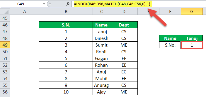
The succeeding table shows the serial number (S.N.), name, and department of ten employees in an organization. We want to find the serial number of the employee “Tanuj.”
We apply the following formula.
“=INDEX(B46:D56,MATCH(G48,C46:C56,0),1)”
The MATCH function searches for the exact word “Tanuj” in the range C46:C56 and returns 2. The output 2 is supplied as the row number to the INDEX function. The INDEX function returns the value from the second row and first column of the range B46:D56.
The output of the formula is 1. This implies that the serial number of “Tanuj” is 1.
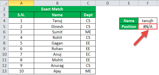
The following image shows the output when the “lookup_value” is “Tanujh.” Since “Tanujh” could not be found in column B, the outcome is “#N/A” error.
The Properties of the MATCH Excel Function
- It is not case-sensitive which implies that it does not distinguish between the uppercase and lowercase letters.
- It returns the relative position of the “lookup_value” in the “lookup_array.”
- It works with one-dimensional ranges or arrays which can be either vertical or horizontal.
- If there are multiple occurrences of the “lookup_value” in the “lookup_array,” it returns the position of the first exact match.
- If the “lookup_value” is in text form, the wildcard characters like a question mark (?) and asterisk (*) can be used for partial matches.
- It returns the “#N/A” error if it is unable to find the “lookup_value” in the “lookup_array.”
Frequently Asked Questions (FAQs)
1. Define the MATCH function of Excel.
The MATCH function returns the position of a given value from a vertical or horizontal array or range of cells. It returns both approximate and exact matches from unsorted and sorted data lists respectively.
The MATCH function can be used in combination with the INDEX function to extract a value from the position supplied by the former. The MATCH function accepts the arguments “lookup_value,” “lookup_array,” and “match_type.”
The first two arguments are mandatory, while the last is optional. The “match_type” can take the values 1, 0 or -1 depending on the type of match. The value 0 refers to an exact match, while 1 and -1 refer to an approximate match.
2. How is the MATCH function used to compare two columns in Excel?
The MATCH function is used in combination with the IF and ISNA functions to compare two columns. The formula is stated as follows:
“IF(ISNA(MATCH(first value in list1,list2,0)),“not in list 1”,“”)”
The formula looks for a value of “list 1” in “list 2.” If it is able to find a value, its relative position is returned. However, if a value of “list 2” is not present in “list 1,” the formula returns the text “not in list 1.”
3. What is the INDEX MATCH formula of Excel?
The INDEX MATCH formula uses a combination of the INDEX and MATCH functions. The INDEX function looks for a value in an array based on the specified row and column numbers. These row and column numbers are supplied by the MATCH function.
The INDEX MATCH formula for a vertical lookup is stated as follows:
“INDEX(column to return a value from,MATCH(lookup_value,column to look up against,0)”
The “column to return a value from” is the “array” argument of the INDEX function. The “column to look up against” is the “lookup_array” argument of the MATCH function.
Note: The “array” argument of the INDEX function must contain the same number of rows as the “lookup_array” argument of the MATCH function.
Recommended Articles
This has been a guide to the MATCH function in excel. Here we discuss how to use Match Formula along with step by step excel example. You can download the Excel template from the website. Take a look at these lookup and reference functions of Excel-