AGGREGATE Excel Function

The AGGREGATE function of Excel returns the aggregate of a given data table or data list. The first argument is a function number, and the further arguments consist of a range of data sets. One must remember the function number to know which function to use.

• AGGREGATE function in Excel returns the aggregate of data provided in a table or data list.
• In the AGGREGATE function, the first argument is function number, and further arguments are for a range of the data sets.
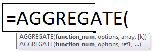
• The reference syntax of the AGGREGATE formula is “=AGGREGATE(function_num, options, ref1, ref2, ref,…)”
• The Array syntax of AGGREGATE formula is “=AGGREGATE(function_num,options,array,)”
• “k” is an optional argument used with functions like LARGE, SMALL, PERCENTILE.EXC, QUARTILE.INC, PERCENTILE.INC, and QUARTILE.EXC.
• The AGGREGATE function is often used to replace different functions for different conditions without using the conditional formula.

The two syntaxes of the function are stated as follows:

Array Syntax

“=AGGREGATE(function_num,options,array,)”

Reference Syntax

“=AGGREGATE(function_num,options, ref1, ref2, ref,…)”

The function accepts the following arguments:

Function_num: This number represents a specific function that is to be used. It ranges from 1-19.

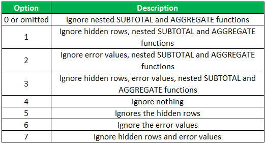
Options: This is a numeric value ranging from 0 to 7. It determines the values that are ignored during calculations.

Ref1, ref2, ref: This is the numeric value or values on which computations are to be performed.

It is mandatory to provide at least two of these arguments, and the remaining arguments are optional.

The features of the AGGREGATE function are listed as follows:

• It does not recognize the function_num value greater than 19 and lesser than 1.
• For Option Number, the AGGREGATE function does not identify the values greater than 7 and lesser than 1.
• If we feed any other values, it gives a “#VALUE! error.”
• It always accepts a numeric value and always returns a numeric value as the output.
• It ignores only the hidden rows but does not ignore the hidden columns.

Example #1

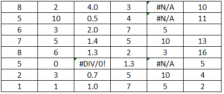
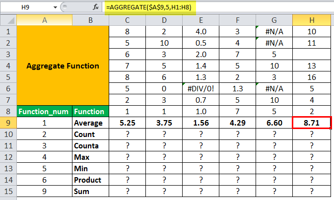
We have a list of numbers, and we want to compute the Average, Count (the number of cells that contain a value), Counta (count of cells that are not empty), Maximum, Minimum, Product, and Sum. The values are given in the following table:

Let us first calculate the Average in the ninth row for all the given values. For Average, the function_ num is 1.

The values are given in column C. Since no values are ignored, we select option 4 (i.e., ignore nothing).

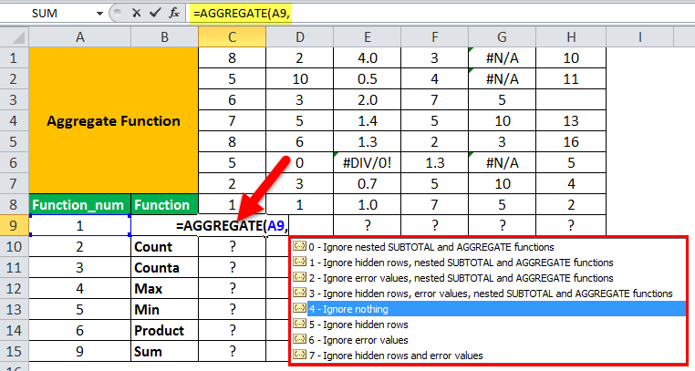
We select the range of values C1:C8.

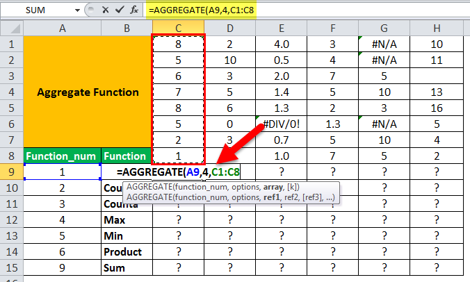
We calculate the Average by omitting the value of “k.”

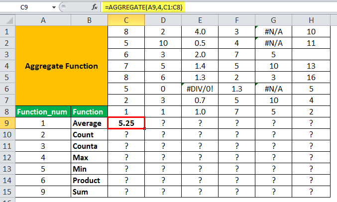
The average value is 5.25, as shown in the succeeding image.

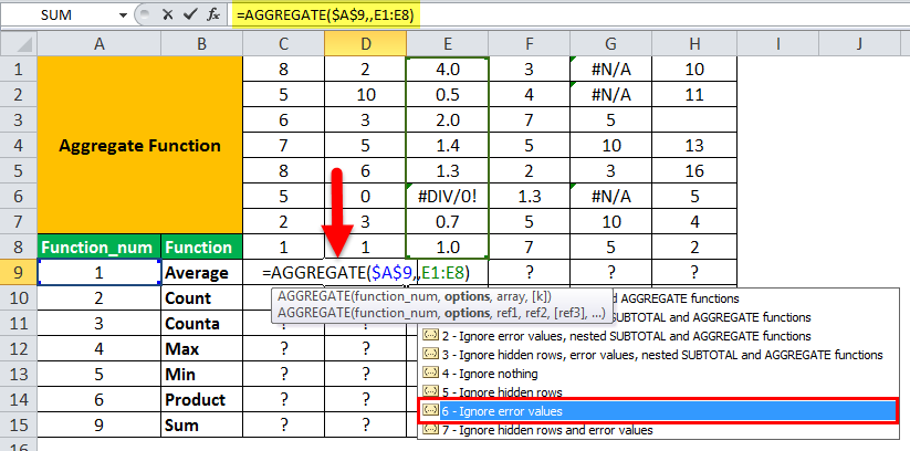
Similarly, for range D1:D8, we select option 4.

In range E1:E8, cell E6 contains an error value. If we use the same AGGREGATE formula, we get an error. If an appropriate option is used, the AGGREGATE function gives the average of the remaining values while neglecting the error in E6.

To ignore the error values, we select option 6.

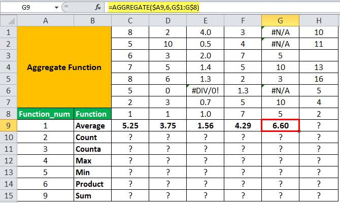
Similarly, for range G1:G8, we use option 6 (ignore the error values).

For cell H3, we enter the value 64, hide the third row, and use option 5 to ignore the hidden row. The AGGREGATE function gives the average value of the numeric values that are visible.

The output without hiding the third row is shown in the succeeding image.

The output after hiding the third row is shown in the succeeding image.

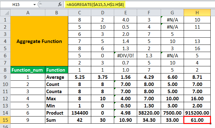
We apply the AGGREGATE formula to other operations, as shown in the following image.

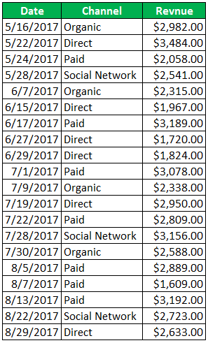
Example #2

A table shows the revenue generated on different dates from the different channels. We want to find the revenue generated from the different channels.

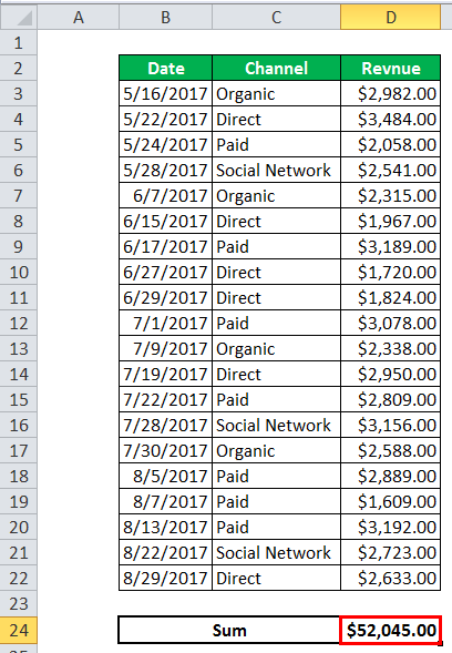
We apply the SUM function to get the total revenue generated.

If we want to check the revenue generated from “Organic Channel” or “Direct Channel,” we apply filters in Excel. The SUM function gives the total sum.

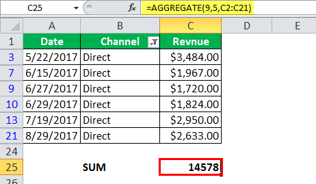
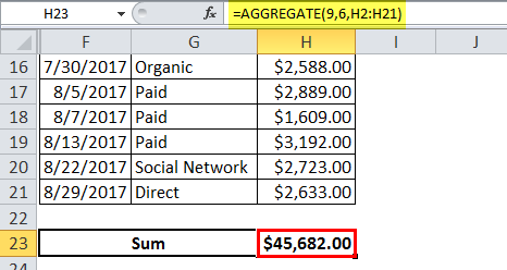
To get the sum of the visible values when a filter is applied, instead of using the SUM function, we will use the AGGREGATE function. So, on replacing the SUM formula with an AGGREGATE function with option code 5 (ignoring the hidden rows and values); we have,

We apply the filter to different channels. It shows the sum of revenue for the filtered channel. The rest of the rows are hidden.

Total Revenue Generated for Direct Channel is shown in the succeeding image:

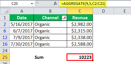
Total Revenue Generated for Organic Channel is shown in the succeeding image:

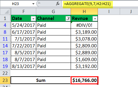
Total Revenue Generated for Paid Channel is shown in the succeeding image:

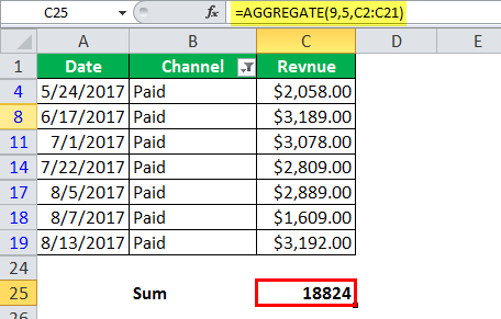
The AGGREGATE function calculates the different SUM values for the revenue generated from different channels. The AGGREGATE function is dynamic in nature. It is used to replace different functions for different conditions without using the conditional formula.

Let us assume that in the same table, some of the revenue values contain an error. We want to ignore the errors. At the same time, if we apply a filter, the AGGREGATE function should ignore the hidden row values.

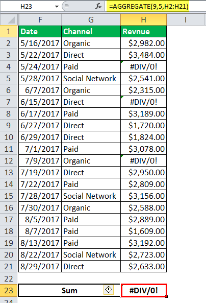
When we use option 5, we get an error as the sum of the total revenue. With the usage of option 6, the SUM function ignores error values.

When we apply the filter (for example, filter by channel value Direct), the SUM function ignores the errors. However, we also need to ignore the hidden values.

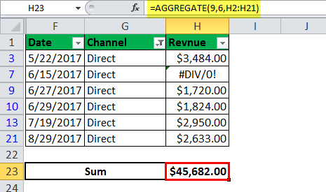
In this case, we use option 7. This ignores the error values and the hidden rows simultaneously.

Guide to the AGGREGATE function in Excel. Here, we discuss how to use AGGREGATE formula along with step by step example. You may also look at these useful functions in Excel –

• REPLACE Function in Excel
• POWER Function in Excel
• IF Function
• True Function in Excel