#1 Freeze the First Column in Excel
Freezing the first column locks column A of the worksheet. This means that on moving from left to right, this column will be visible at all times.
Remove Watermark Excel Template
Download Excel TemplateIn addition, column A is fixed irrespective of the column from which the actual data begins. The excel shortcut to freeze the first column is “Alt+W+F+C” (when pressed one by one).

Let us consider an example.
Example #1
The following table shows the sales revenue (in $) generated by the products of specific segments. The data relates to various countries and is spread across the first five months of the year 2015.
We want to freeze the first excel column (column A).

In order to view the column “segment” on a movement from left to right, we need to freeze it.
The steps for freezing the excel column are listed as follows:
- Select the worksheet where the first column is to be frozen.
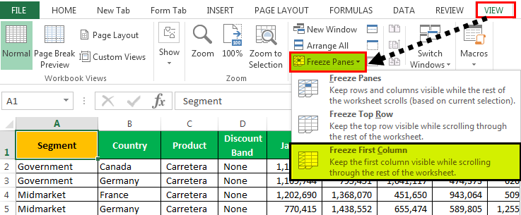
- In the View tab, click the “freeze panes” drop-down under the “window” section. Select “freeze first column,” as shown in the succeeding image.
Alternatively, press the shortcut keys “Alt+W+F+C” one by one.

- The first column is frozen. The grey line appears at the end of column A indicating that the column to the left is frozen. The column AB shown in the following image is the last scrolled column of the dataset.

- On scrolling (from left to right) through the remaining columns of the dataset, column A is visible. The same is shown in the following image.


In the same way, the first row can be frozen.
#2 Freeze Multiple Columns in Excel
Freezing multiple excel columns is similar to freezing multiple rows. For freezing multiple columns, select the first right-hand side cell immediately after the last column to be frozen. This is because multiple columns are frozen based on the current selection.
Similarly, for freezing multiple rows, select the first cell immediately below the last row to be frozen.
For example, to freeze the columns A, B, and C, select the cell D1. By freezing the first three columns, they remain visible to the user at all times. Likewise, to freeze the rows 1, 2, and 3, select the cell A4.
The shortcut to freeze multiple excel columns is “Alt+W+F+F” (when pressed one by one).

Let us consider an example.
Example #2
Working on the data of example #1, we want to freeze the first four columns, A, B, C, and D.
The steps for freezing multiple excel columns are listed as follows:
Step 1: Select the cell E1. This is because the first four columns are to be frozen.

Step 2: In the View tab, click the “freeze panes” drop-down under the “window” section. Select “freeze panes,” as shown in the succeeding image.
Alternatively, press the shortcut keys “Alt+W+F+F” one by one.

Step 3: The first four columns are frozen. The grey line appears (shown in the following image) at the end of column D, indicating that the columns to the left are frozen.
The columns R and S shown in the following image are the scrolled columns towards the end of the dataset.

Step 4: On scrolling (from left to right) till the last column of the dataset, the first four columns are visible. The same is shown in the following image.
#3 Freeze the Row and Column Together in Excel
Usually, the first row and the first column of a database contain headers. The user might want to view the row 1 and the column A simultaneously and at all times. Hence, it is essential to lock them together to permit their visibility while scrolling down and from left to right.
The only difference between the methods #2 and #3 is in the selection of the cell (step 1). With the “freeze panes” option, Excel freezes the rows and columns preceding the current active cell.
The shortcut to freeze the row and column together is “Alt+W+F+F” (when pressed one by one).
Let us consider an example.
Example #3
Working on the data of example #1, we want to freeze the first row (row 1) and the first column (column A) at the same time.

The steps to freeze the excel row 1 and column A together are listed as follows:
Step 1: Select the cell B2.

Step 2: Press the shortcut keys “Alt+W+F+F” one by one. It freezes the column to the left of the selected cell B2. At the same time, the row preceding the active cell (B2) is also frozen, as shown in the following image.
Hence two grey lines appear, one at the end of row 1 (horizontal) and the other at the end of column A (vertical).
Note: Alternatively, the “freeze panes” option can be selected from the “freeze panes” drop-down of the View tab.

Step 3: On scrolling from top to bottom and left to right, the row 1 and column A are visible. The same is shown in the following image.
Note: It is possible to freeze as many rows and columns depending on the requirement. The condition is that freezing of multiple excel rows and columns should begin with the top row (row 1) and the first column (column A).

#4 Unfreeze Panes in Excel
Unfreezing of panes does not require any cells to be selected. The steps to unfreeze panes in Excel are listed as follows:
Step 1: In the View tab, click the “freeze panes” drop-down under the “window” section. Select “unfreeze panes,” as shown in the succeeding image.
Alternatively, press the shortcut keys “Alt+W+F+F” one by one.

Step 2: The grey lines are removed, as shown in the following image.
Note: The “unfreeze panes” option appears only after freezes have been applied to the Excel worksheet.

The Rules of Freezing in Excel
The norms governing the freezing of rows and columns are listed as follows:
- It is not possible to freeze excel rows and columns in the middle of the worksheet.
- The option “freeze panes” can be applied only once. It is not possible to create multiple “freeze panes” in a single worksheet.
- The rows and columns to be fixed should be visible at the time of freezing. Otherwise, they will remain hidden even after freezing.
Note 1: To divide a worksheet into two or more areas with separate scroll bars for each, use the “split” option. This is available in the “window” section of the View tab.
Note 2: To fix the header row of a large dataset that does not fit into the screen, create an Excel table. Moreover, ensure the visibility of this row by selecting any cell within the table before scrolling.
Frequently Asked Questions
1. What does freezing columns mean and how to freeze the first column in Excel?
Freezing a column means locking it in order to keep it visible while the user scrolls through the database. This is specifically helpful if a column contains headers which are required to be seen at all times.
After freezing, a grey line appears to indicate the frozen columns on its left. The steps to freeze the first column (column A) are listed as follows:
• In the View tab, click the “freeze panes” drop-down under the “window” section.
• Select “freeze first column.” Alternatively, press the shortcut keys “Alt+W+F+C” one by one.
• The first column (column A) is frozen.
Note: For freezing the first row, select “freeze top row” from the “freeze panes” drop-down of the View tab.
2. How to freeze multiple columns in Excel?
Let us freeze columns A, B, C, D, and E. The steps to freeze multiple columns in Excel are listed as follows:
• Select either the column or the first cell to the right of the last column to be frozen (column E). So, select either column F or the cell F1.
• In the View tab, click the “freeze panes” drop-down under the “window” section.
• Select “freeze panes.” Alternatively, press the shortcut keys “Alt+W+F+F” one by one.
• The columns A B, C, D, and E are frozen as indicated by the grey line at the end of column E.
3. How to freeze rows and columns together in Excel?
Let us freeze rows 1, 2, and 3 and columns A, B, and C. The steps to freeze the given rows and columns together are listed as follows:
• Select cell D4 based on the following parameters:
a. It immediately follows the last row to be frozen (row 3).
b. It is to the right of the last column to be frozen (column C).
• In the View tab, click the “freeze panes” drop-down under the “window” section.
• Select “freeze panes.” Alternatively, press the shortcut keys “Alt+W+F+F” one by one.
• The rows 1, 2, and 3 and columns A, B, and C are frozen. This is indicated by the grey line appearing below row 3 and at the end of column C.
Note: The freezing of multiple excel rows and columns should begin with the top row (row 1) and the first column (column A).
Recommended Articles
This has been a guide to freezing columns in Excel. Here we discuss how to freeze the first column, multiple columns, and both rows and columns. For more on Excel, take a look at the following articles-