VBA Worksheet Function

Worksheet function in VBA one may use when we have to refer to a specific worksheet. Normally, when we create a module, the code executes in the currently active sheet of the workbook. Still, if we want to execute the code in the specific worksheet, we use the Worksheet function. This function has various uses and applications in VBA.

The best thing about VBA is how we use formulas in worksheets. Similarly, VBA too has its functions. However, if this is the best, it also has a beautiful thing. That is, "we can also use Worksheet functions in VBA."

You heard it right. We can access Worksheet functions in VBA also. We can access some of the worksheet functions while writing and making them part of our code.

In the worksheet, all the formulas start with equal (=) sign, similarly, in VBA coding, to access worksheet formulas, we should use the word "WorksheetFunction."

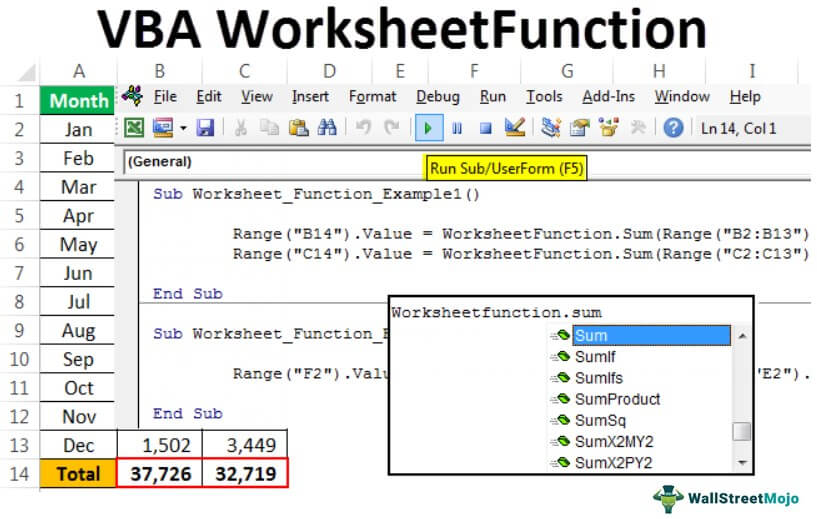
Before entering any worksheet formula, you need to mention the "WorksheetFunction" object name, put a dot (.), and get a list of all the available functions under this object.

In this article, we will exclusively concentrate on how to use Worksheet functions in VBA coding, which will add more value to your coding knowledge.

#1 - Simple SUM Worksheet Functions

To start with Worksheet functions, apply the simple SUM function in excel to add numbers from the worksheet.

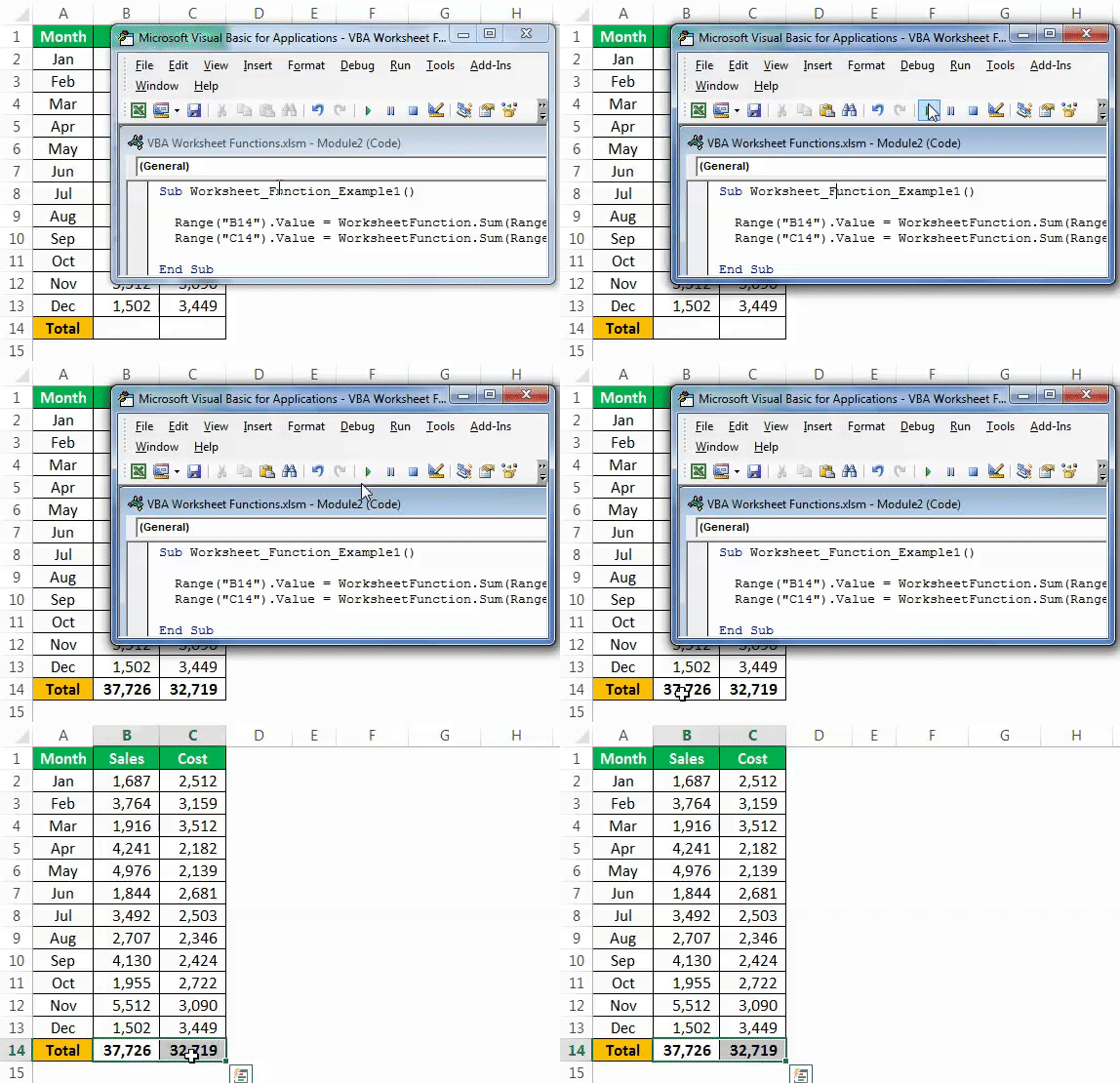
Assume you have monthly sales and cost data in the worksheet like the below one.

In B14 and C14, we need to arrive at the total of the above numbers. Follow the steps below to start applying the SUM function in Excel VBA.

Step 1: Create a simple, excel macro name.

Code:

Sub Worksheet_Function_Example1()

End Sub

Step 2: Since we need the result in cell B14, start the code as Range ("B14").Value =

Code:

Sub Worksheet_Function_Example1()

  Range("B14").Value =

End Sub

Step 3: In B14, we need the value as the result of the sum of the numbers. So to access the SUM function from the worksheet, start the code as "WorksheetFunction."

Code:

Sub Worksheet_Function_Example1()

Range("B14").Value = WorksheetFunction.

End Sub

Step 4: The moment you put a dot (.), it will start to display the functions available. So, select SUM from this.

Code:

Sub Worksheet_Function_Example1()

   Range("B14").Value = WorksheetFunction.Sum

End Sub

Step 5: Reference the above numbers: Range ("B2:B13").

Code:

Sub Worksheet_Function_Example1()

  Range("B14").Value = WorksheetFunction.Sum(Range("B2:B13"))

End Sub

Step 6: Similarly, for the next column, apply a similar code by changing the cell references.

Code:

Sub Worksheet_Function_Example1()

  Range("B14").Value = WorksheetFunction.Sum(Range("B2:B13"))
  Range("C14").Value = WorksheetFunction.Sum(Range("C2:C13"))

End Sub

Step 7: Run this code manually or use the F5 key to have a total in B14 and C14 cells.

We got our values. You need to notice that we don't have any formula in the worksheet, but we just got the result of the SUM function in VBA.

#2 - Use VLOOKUP as a Worksheet Function

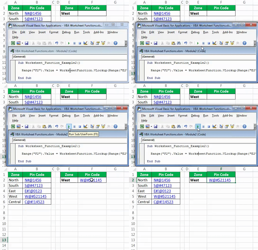
We will see how to use VLOOKUP in VBA. Assume below is the data you have in your Excel sheet.

In the E2 cell, you had created a drop-down list of all the zones.

Based on the selection you made in the E2 cell, we need to fetch the pin code for the respective zone. But this time, through VBA VLOOKUP, not worksheet VLOOKUP. So, follow the below steps to apply VLOOKUP.

Step 1: Create a simple Macro name in the sub procedure.

Code:

Sub Worksheet_Function_Example2()

End Sub

Step 2: We need the result in the F2 cell. So start the code as Range ("F2").Value =

Code:

Sub Worksheet_Function_Example2()

  Range ("F2").Value =

End Sub

Step 3: To access the worksheet function, VLOOKUP starts the code as "WorksheetFunction.VLOOKUP."

Code:

Sub Worksheet_Function_Example2()

  Range ("F2").Value = WorksheetFunction.Vlookup(

End Sub

Step 4: One of the problems here is syntax will not guide you to work with VLOOKUP. It would help if you knew the syntax you were working on.

The first syntax of VLOOKUP is "Lookup Value." In this case, our lookup value is the E2 cell, so write the code as  Range (“E2”).Value

Code:

Sub Worksheet_Function_Example2()

  Range ("F2").Value = WorksheetFunction.Vlookup(Range ("E2").Value,

End Sub

Step 5: Now, the second argument is our table array. In this case, our table array range is from A2 to B6. So the code will be Range ("A2:B6").

Code:

Sub Worksheet_Function_Example2()

  Range ("F2").Value = WorksheetFunction.Vlookup(Range ("E2").Value,Range ("A2:B6"),

End Sub

Step 6: The third argument will be from which column we need the data from the table array. Here we need the data from the second column so that the argument will be 2.

Code:

Sub Worksheet_Function_Example2()

  Range ("F2").Value = WorksheetFunction.Vlookup(Range ("E2").Value,Range ("A2:B6"),2,

End Sub

Step 7: The final argument is range lookup, we need an exact match, so the argument is zero (0).

Code:

Sub Worksheet_Function_Example2()

  Range("F2").Value = WorksheetFunction.VLookup(Range("E2").Value, Range("A2:B6"), 2, 0)

End Sub

So, we have completed the coding part. Now, go to the Worksheet and select any of the ranges.

Now, go to your coding module and run the Macro using the F5 key or manually to get the pin code of the selected zone.

We cannot go back and run the Macro every time, so let's assign a Macro to shapes. Then, insert one of the shapes into a worksheet.

Add a text value to the inserted shape.

Now, right-click and assign the Macro name to this shape.

Click on "OK" after selecting the Macro name.

Now, this shape holds the code of our VLOOKUP formula. So whenever you change the zone name, click on the button to update the values.

• To access worksheet functions, we need to write the word "WorksheetFunction" or "Application.WorksheetFunction"
• We do not have access to all the functions, only a few.
• We do not see the actual syntax of Worksheet functions, so we must be sure of the function we are using.