Pivot Table Update

Last Updated :

21 Aug, 2024

Blog Author :

Edited by :

Reviewed by :

Table Of Contents

What Is Update Pivot Table In Excel?

Pivot Table Update in Excel is a method used to update the already created pivot table if any changes are made to the original table. Updating pivot table, in simple terms, means refreshing the pivot table. But, this refresh is a manual process.

For example, consider the below pivot table. It shows the grand total of various sample products and the sales as shown in the below image.

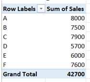
Now, assume the sales of sample F is changed from 7600 to 6000 dollars. To make sure the grand total is also changed accordingly, we have to right-click on the pivot table and click on Refresh.

We can see the pivot table showing updated results.

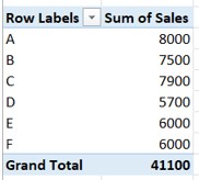
Likewise, we can update pivot table in Excel.

In this article, we will show you how to update the PivotTables.

What Is Update Pivot Table In Excel?

Pivot Table Update in Excel, as the name suggests updates the already created pivot table.
Changes include insertion, deletion or alteration of values in the original Excel table data.
Updating pivot table in Excel is a manual process.
Users can easily refresh or update the pivot table in Excel by right-clicking the pivot table and clicking on Refresh button.
In case, the refresh button is not working, we can click on Change Data Source under PivotTable analyze tab in Excel.

How To Update Pivot Table?

The steps to update the PivotTable are as follows:

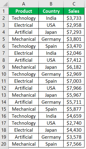
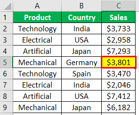
For example, look at the below data in an excel worksheet.
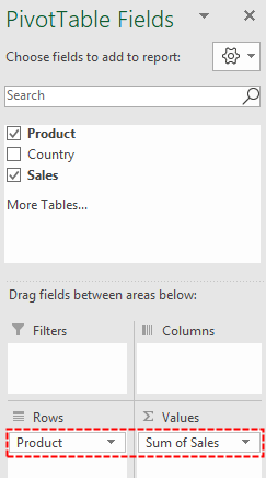
We will summarize this report by adding a PivotTable. So, let us insert a PivotTable first.
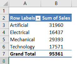
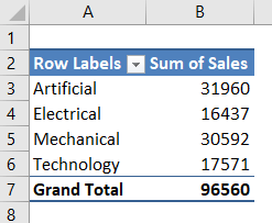
Our PivotTable looks like, as shown below.
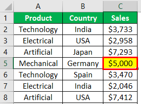
Ok, now we will go to the primary data and change one of the sales numbers.
Cell C5’s current value is $3,801 and will change to $5,000.
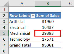
If you return to the Excel PivotTable and see the result for “Mechanical” remains the same as the old one is 29393.

So, this is the problem with a PivotTable.
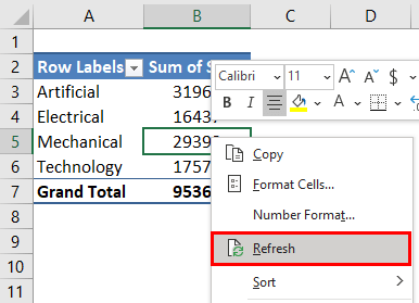
To update the report to show updated results, right-click on any of the cells inside the PivotTable and choose the option of “Refresh.”
Upon refreshing the report, we can see updated results now.

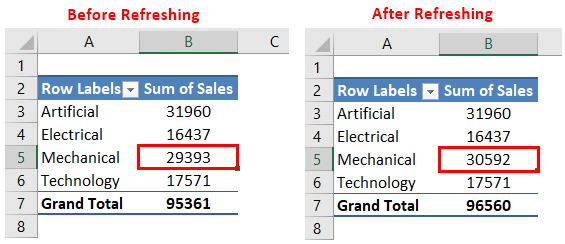
Now, look at the result of the PivotTable. Before refreshing, we had a value of 29393 for the product “Mechanical.” After refreshing, it shows 30592.

Like this, we can refresh the PivotTable if there are any changes in the existing data set.

Update Pivot Table If Any Addition To The Existing Data Set

We have seen how we can refresh the PivotTable if the data numbers of the existing data set change, but this is not the same if their addition to the current data set.

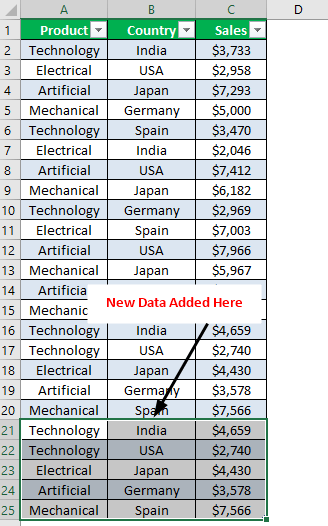
We will add five more data lines for an example of the above existing data set.

If you go and refresh the PivotTable, it will not consider the additional data.

That is because while creating the PivotTable, it has taken the data range reference of A1:C20. However, since we added data after row 20, it would not automatically grab the data range.

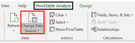
To view the data range reference in the PivotTable sheet, select any of the cells of the PivotTable. It will open up two more tabs in the ribbon: “PivotTable Analyze” and “Design,” respectively. Under the “PivotTable Analyze” tab, click on the “Change Data Source” option.

It will take us to the datasheet with the already selected data range.

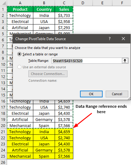
As we can see above, the existing PivotTable has taken the data range reference as A1:C20; since we added the new data after row number 20. So, it would not show even after refreshing the PivotTable. So, it would not show the newly updated result.

So, we need to select the new data range in the above window, so choose the new data range from A1:C25.

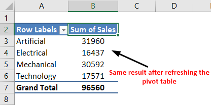
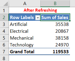
Click “OK.” Our PivotTable will show the updated results.

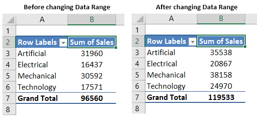
As we can see above, after changing the data range, our PivotTable shows the new results, so anything that happens to the range of cells from A1:C25 will be reflected upon refreshing.

Auto Data Range For Pivot Table With Excel Tables

As we have seen above, we needed to change the data range manually in case of additional data but using Excel tables. We can make the data range automatically picked for a PivotTable.

First, convert the data range to an Excel table by pressing “Ctrl + T.“

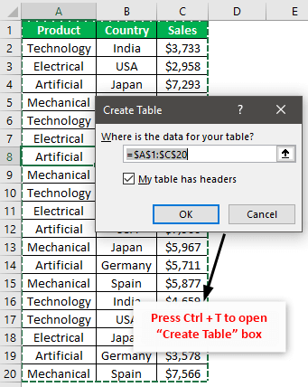
Click “OK.” It will convert our data range to “Excel Table.”

Now, create a PivotTable by selecting the Excel Table range.

Now, go to data and add a few lines of data after the last row of the existing data range.

Now, return and refresh the PivotTable to get the result.

Like this, we can use different techniques to update the PivotTable in Excel.

Update Multiple Pivot Table Results Using Shortcut Keys

Imagine 10 to 20 PivotTables. Can you update the PivotTable by going to each PivotTable and pressing the “Refresh” button?

It is highly time-consuming. Instead, we can rely on a single shortcut key to update all the PivotTables in the workbook.

It will refresh all the PivotTables in the workbook.

Important Things To Note

If the data range is a standard reference, then the PivotTable will not consider additional data.
By converting the data range to excel tables, we can make the data range reference normal.

Frequently Asked Questions

1. What is Pivot table update in Excel?

PivotTables are great for analyzing large amounts of data. It will help us greatly tell the story behind the data. However, there is a limitation with a PivotTable. If there are any changes in the existing data or any addition or deletion of the data, then the PivotTable cannot show the reports instantly. Hence, it requires the user’s intervention to show updated results.

2. Explain how to update pivot table with an example.

For example, consider the below pivot table. It shows the grand total of various products and the sales as shown in the below image.

FAQ 2

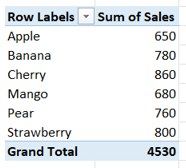
Now, assume the sales of strawberry is changed from 800 to 900 dollars. To make sure the grand total is also changed accordingly, we have to right-click on the pivot table and click on Refresh.

We can see the pivot table showing updated results.

Pivot Table Update - FAQ 2 - Output

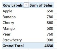
Likewise, we can update pivot table in Excel.

3. How to update pivot table in Excel?

Updating Pivot Table in Excel is a manual process. We can simply refresh the pivot table or click on Change Data Source under PivotTable analyze.