Pivot Table Filter

Last Updated :

21 Aug, 2024

Blog Author :

Edited by :

Reviewed by :

Table Of Contents

What Is Pivot Table Filter?

Pivot Table Filter is a filter that is applied to the generated Pivot Table to highlight or focus a specific portion of data. These are not similar to the data validation filters we use in the Excel worksheets. We can also use the Pivot Table Slicer option to filter and separate the required data from a Pivot Table.

For example, when we apply the Pivot Table Filter on a generated Pivot Table, we get the option to filter the required data, as shown below.

Pivot Table Filter - Example

Table of contents

What Is Pivot Table Filter?
The Pivot Table filter helps us to filter and project only the required data in a large dataset. When we apply the filter, we can always remove the filter at any point in time to get back the full data.
The Pivot Table filtering is not an additive because when we filter one criteria and want to apply the filter again for another criteria, the first one will get discarded.
In this filter, when we use the CSV method, we use the TEXTJOIN function, a new formula introduced in Excel 2016. However, if it is not found, we can always use the CONCATENATE function, as it, too, makes the text-joining process much easier.

How To Filter In A Pivot Table?

We can Filter Pivot Table using two methods,

Right-click on the Pivot Table, and click the “Filter” option.
Use the filter options provided in the Pivot Table fields.

Features like Pivot Table Filter and other advanced tools in Excel allow users to analyze complex data, automate tasks, and use advanced functions. Those looking to improve their data management skills using Excel can explore this Advanced Excel Functions Course.

Let us look at multiple ways of using a filter in an Excel Pivot table: -

#1 - Inbuilt filter in the Excel Pivot Table

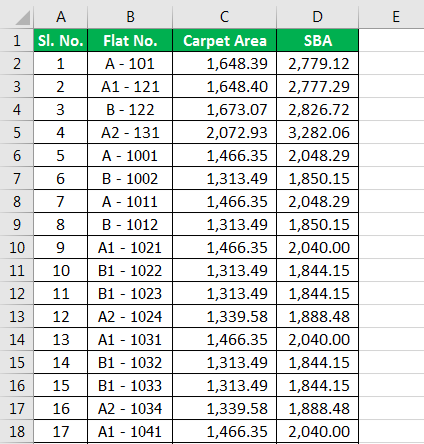
Consider the data given below that has Serial numbers, Flat Number, Carpet Area, and SBA.

Pivot table Filter examplee 1.1

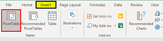
Go to the “Insert” tab, and select a Pivot Table, as shown below.

Pivot table Filter examplee 1.2

The “Create a Pivot Table” window pops out when you click on the Pivot Table.

Pivot table Filter examplee 1.3

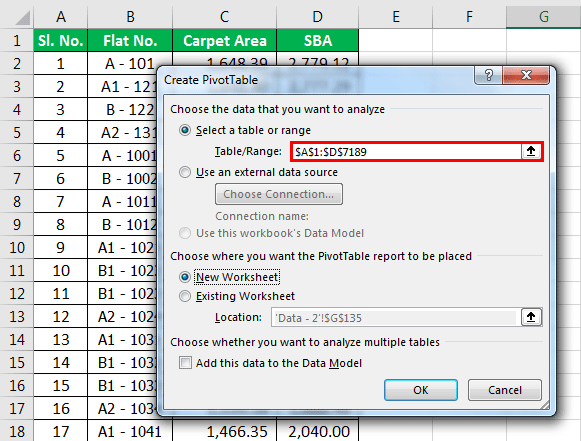
In this window, we can select a table or a range to create a Pivot Table. Else, we can also use an external data source.

We can also place the Pivot Table report in the same worksheet or a new one.

For example, we can see this in the above picture.

The “Pivot Table Fields” is available on the right end of the sheet as below.

Pivot table Filter examplee 1.4

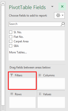
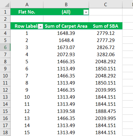
We can observe the filter field, where we can drag the fields into filters to create a Pivot Table filter. Let us drag the “Flat.No” field into “Filters.” We can see the filter for flat no’s would have been created.

Pivot table Filter examplee 1.5

From this, we can filter the flat numbers as per our requirement, which is the normal way of creating the filter in the Pivot Table.

Pivot table Filter examplee 1.6

#2 - Create a filter for the Values Area of an Excel Pivot Table

Generally, when we take data into value areas, we will not create any filter for those Pivot Table fields. However, we can see it below.

Pivot table Filter examplee 2.1

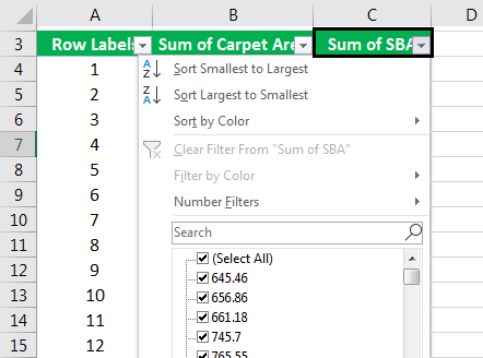
We can observe that there is no filter option for value areas: Sum of SBA and Sum of Carpet Area. But we can create it, which helps us in various decision-making purposes.

Pivot table Filter examplee 2.2

Firstly, we must select any cell next to the table and click on the “Filter” in the “Data” tab.

Pivot table Filter examplee 2.3

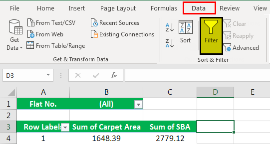
We can see the filter gets in the “Values” area.

Pivot table Filter examplee 2.4

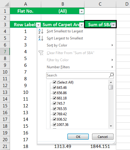
As we get the filters, we can perform different types of operations from value areas, like sorting them from largest to smallest to know top sales/area/anything. Similarly, we can sort from smallest to largest, sorting by color, and even perform number filters like <=, < , >=, >, and many more. So, it plays a major role in decision-making in any organization.

#3 - Display a list of multiple items in a Pivot Table Filter

The above example taught us about creating a filter in the Pivot Table. Now, let us look at how we display the list differently.

The three most important ways of displaying a list of multiple items in a Pivot Table filter are:

Using Slicers.
Creating a list of cells with filter criteria.
List of comma-separated-values.

#4 - Using Slicers

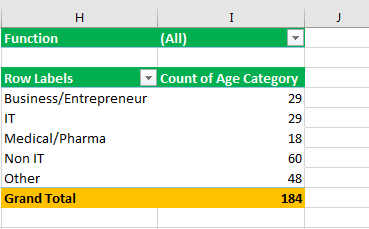
Let us have a simple Pivot Table with columns: Region, Month, Unit no, Function, Industry, and Age Category.

example 3.1

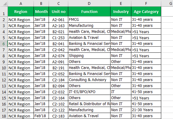
First, create a Pivot Table using the above-given data. Then, select the data, go to the “Insert” tab, select a “Pivot Table” option, and create a Pivot Table.

example 3.2 example 3.4

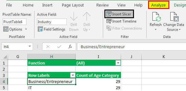
From this example, we will consider the function of our filter. First, let us check how it can be listed using slicers and varies as per our selection. It is simple: We select any cell inside the Pivot Table, go to the “Analyze” tab on the ribbon, and choose the “Insert Slicer.”

example 3.3

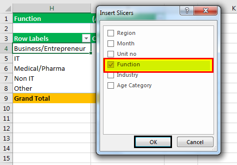
Then, we need to insert the slide in the slicer of the field in our filter area. So, in this case, we must select the “Function” field in our filter area and then press the “OK” button, which will add a slicer to the sheet.

example 3.5

We can see items highlighted in the slicer are those highlighted in our Pivot Table filter criteria in the filter drop-down menu.

example 3.6

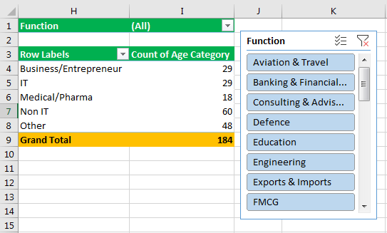
Now, this is a pretty simple solution that does display the filter criteria. By this, we can easily filter out multiple items and can see the result varying in value areas. From the below example, it is clear that we had selected the functions that are visible in the slicer and can find out the count of age categories for different industries (which are row labels that we had dragged into the row label field), which are associated with those functions that are in a slicer. We can change the function per our requirement and observe that the results vary as per the selected items.

However, suppose you have many items on your list here, which is long. In that case, we might not display those items properly. You might have to scroll to see which items are selected, leading us to the next solution: list the filter criteria in cells.

So, “Create List of Cells With Pivot Table Filter Criteria” comes to our rescue.

#5 - Create a List of cells with Pivot Table Filter Criteria

We will use a connected Pivot Table and the above slicer here to connect two Pivot Tables.

Let us create a duplicate copy of the existing Pivot Table and paste it into a blank cell.

example 4.1

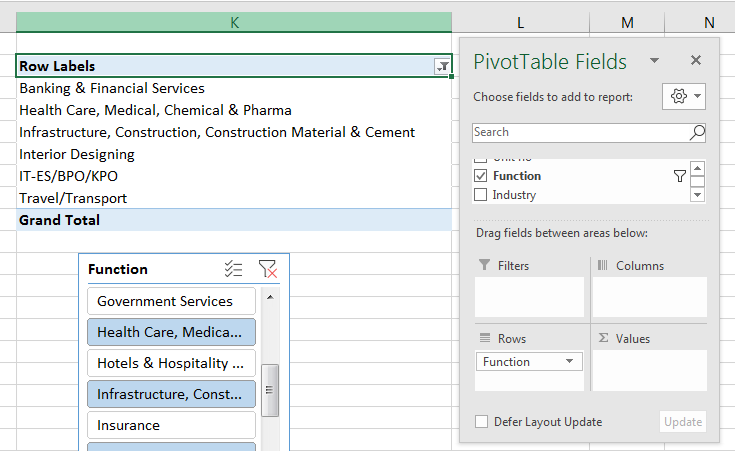
So, we have a duplicate copy of our Pivot Table, and we will modify it slightly to show the “Function” field in the “Rows” area.

To do this, we must select any cell inside our Pivot Table here, go to the Pivot Table field list, and remove industry from the “Rows.” Also, removing the “Count of Age” category from the “Values” area, we will take the “Function” that is in our “Filters” area to the “Rows” area. So, now we can see that we have a list of our filter criteria. If we look over here in our filter drop-down menu, we have the list of items in slicers and function filters.

Now, we have a list of our Pivot Table filter criteria. It works because both of these Pivot Tables are connected by the slicer. We can right-click anywhere on the slicer to report connections.

example 4.2

Pivot Table connections will open up a menu showing that these Pivot Tables are connected as checkboxes are checked.

example 4.3

It means whenever one change is made in the first Pivot Table, it automatically gets reflected in the other. We can move Pivot Tables anywhere. For example, we can use it in any financial model and change row labels.

#6 - List of Comma Separated Values in Excel Pivot Table Filter

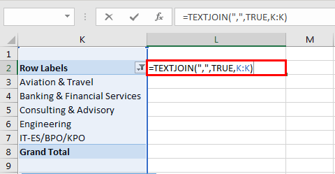
So, the third way to display our Pivot Table filter criteria is in a single cell with a list of comma-separated values. We can do that with the TEXTJOIN function. We still need the tables we used earlier and just used a formula to create this string of values and separate them with commas.

The TEXTJOIN function provides us with three different arguments:

Delimiter – It can be a comma or space.
Ignore empty – TRUE or FALSE to ignore blank cells or not.
Text – Add or specify a range of cells that contain the values we want to concatenate.

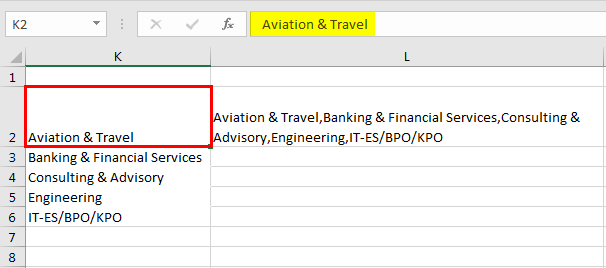
Let us type the TEXTJOIN – (delimiter- which would be “,” in this case, TRUE (as we should ignore empty cells), K: K(like the list of selected items from the filter will be available in this column)to join any value and also ignore any empty value).

Pivot table Filter example 5.1

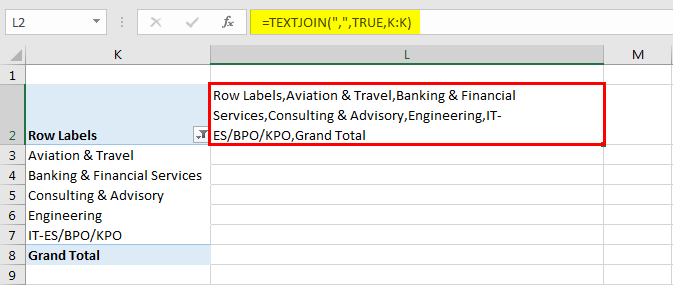
Now, we see getting a list of all our Pivot Table filter criteria joined by a string. So, it is a comma-separated list of values.

Pivot table Filter example 5.2

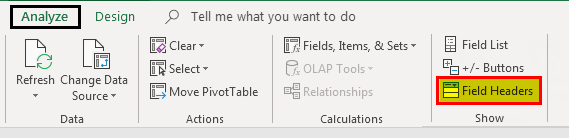
We could hide the cell if we did not want to show these filter criteria in the formula. Select the cell and go to the “Analyze” options tab. Click on “Field Headers,” and that will hide the cell.

Pivot table Filter example 5.3

So, now we have the list of values in their Pivot Table filter criteria. If we change the Pivot Table filter, it reflects in all the methods. We can use any one of them. But eventually, for a comma-separated solution, a slicer and the list are required. We can hide them if we do not want to display the tables.

Pivot table Filter example 5.4

Important Things To Note

We have a special feature in the Pivot Table filter: “Search Box,” which allows us to manually deselect some of the results we do not want. For example, if we have a huge list and there are blanks too, then to select blank, we can easily choose by searching for blanks in the search box rather than scrolling down till the end.
We cannot exclude certain results with a condition in the Pivot Table filter, but we can do it by using the “Label Filter”. For example, if we want to select any product with a certain currency like rupee or dollar, etc., then we can use a label filter – ‘does not contain’ and should give the condition.

Frequently Asked Questions (FAQs)

1. What is a Pivot Table in Excel?

• The Pivot Table are generated tables using an existing dataset that allows us to group or filter data to find largest, smallest, SUM, AVERAGE, COUNT, etc.
• They project the dataset in an organized way where we can only filter the required data and help users track and analyze a large dataset using a compact table.
• It helps to compare data, or show relationships between parameters.
• Apart from the mathematical operations, the Pivot Table has one of the best features: filtering, which allows us to extract defined results from our data.

2. Why is the Pivot Table Filter not working or greyed out?

A few reasons the Pivot Table Filter may not work are,

• The dataset linked to the generated Pivot table is deleted or modified.
• The data modifications are done within the selected dataset, and the Pivot Table is not updated automatically. In such scenarios, refresh the Pivot table manually, to display the current data.

3. What are the uses of Pivot Table Filters?

A few uses of the Pivot Table Filters are as follows:

• In a large dataset, generating a Pivot Table helps us view data in an organized way. And the Pivot Table Filters help us view only the needed data.
• When we use the Pivot Table Slicers to project the Filtered data, we can also format them with different colors to make the data more presentable and understandable.

Download Template

This article must help understand Pivot Table Filter with its features and examples. You can download the template here to use it instantly.

Pivot Table Filter Excel Template