Pivot Table Sort

Last Updated :

21 Aug, 2024

Blog Author :

Edited by :

Reviewed by :

Table Of Contents

What Is Sorting A Pivot Table In Excel?

Sorting a pivot table in Excel option is available in the "Data" tab, and as the name suggests, we can sort the data in the PivotTables. On the PivotTables, right-click on any data we want to sort, and we will get an option to sort the data as we want. The normal sort option does not apply to PivotTables, and PivotTables are not the normal tables. The sorting done from the PivotTable is known as PivotTable Sort.

Sorting means arranging data or certain items in an order, however desired. It can be in ascending or descending order, sorted by values or ranges. At the same time, a PivotTable is a unique tool to summarize data to form a report.

When we generate data, we can arrange it in ascending or descending order in the PivotTable, just like any other cell range where we can sort the data using the AutoFilter tool.

Table of contents

What Is Sorting A Pivot Table In Excel?
PivotTable Sort in the PivotTable is a sorting mechanism. You can sort data in PivotTables by using this sorting option in the "Data" tab or by right-clicking on any data. The normal sort option does not work on PivotTables since they are not normal tables.
To sort data in a PivotTable, we'll need to generate a PivotTable first.
Sorting arranges data in a specific order based on its type. Numeric data can be sorted in ascending or descending order, while strings can be sorted alphabetically.

How To Sort Pivot Table Data In Excel?

Following are the steps used for sorting PivotTable data in Excel: -

First, create a Pivot Table based on data.
Right-click the value to be sorted in the data and select the desired sorting command.

Sorting data in a pivot table is a handy feature. You can definitely use it for better data presentation, analysis, and interpretation. If you want to learn more about these aspects, Data Analysis In Excel course is for you.

Examples

Example #1

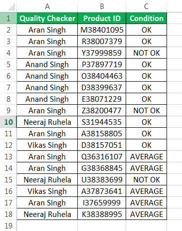
We have data where the quality check department has marked a product "OK" for use and "NOT OK" and "AVERAGE" for use for individual "Product ID." We will build a PivotTable for the data and then find out the highest number of each proportion.

Consider the following data:

Pivot Table sort Example 1

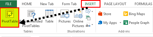
The first step is inserting a PivotTable into the data. Then, in the "Insert" tab under the "Tables" section, click on the "PivotTable." A dialog box appears.

Pivot Table sort Example 1-1

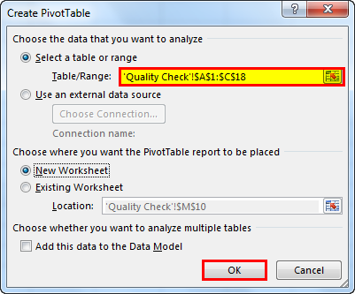
It asks for the data range. We will select the whole data in this process and click on "OK."

Pivot Table sort Example 1-2

We can add a PivotTable either in a new worksheet or in the same worksheet.

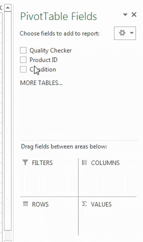
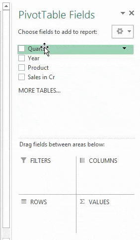
In the new worksheet where the excel takes us, we can see the fields section we discussed earlier. Drag "Condition" in the "Rows" and "Product ID" in the "Values" field.

Pivot Table sort Example 1-3

We can see on the left that the report has been created for the PivotTable.

Pivot Table sort Example 1-4

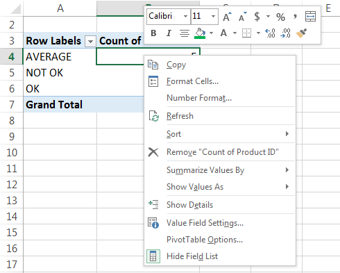
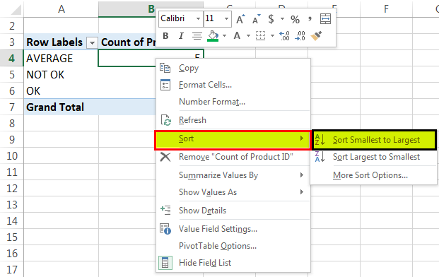
For the current example, we will sort the data in ascending order. Right-click on the "Count of Product ID" column. A dialog box appears.

Pivot Table sort Example 1-5

When we click on "Sort," another section appears. For example, we will click on " Sort Smallest to Largest."

Pivot Table sort Example 1-6

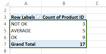
We can see that our data has been sorted in ascending order.

Pivot Table sort Example 1-7

Understanding these principles can significantly impact this approach. This Basic Excel Course is designed to deepen this knowledge and skill set for those eager to build on this foundation.

Example #2

We have data for a company for sales done each quarter by certain products for 2018. We will build a PivotTable over the data and sort the data concerning quarters and the highest number of sales done each quarter.

Have a look at the data below,

Pivot Table sort Example 2

The first step is the same. We need to insert a PivotTable into the data. In the "Insert" tab under the "Tables" section, click on the "PivotTable." A dialog box appears.

Pivot Table sort Example 1-1

As earlier, we need to give it a range. We will select our sales data in the process.

Pivot Table sort Example 2-2

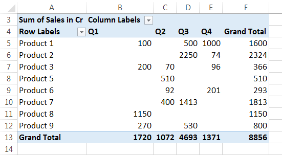
When we click "OK," we may see the PivotTable fields. Now, drag "Quarters" in "Columns," "Product" in "Rows," and "Sales" in "Values."

Pivot Table sort Example 2-3

We have built up our PivotTable for the current data.

Pivot Table sort Example 2-4

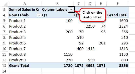
Now, we will first sort the quarters. Then, we will click on the "AutoFilter" in the "Column Labels."

Example 2-5

A dialog box appears where we can see the option to sort the quarter from A to Z or Z to A.

Example 2-6

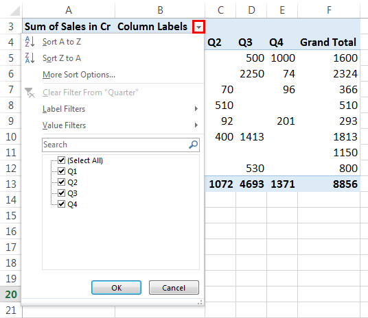
We can choose either of them as to how we want to display our data.
Now, right-click on "Sales." Another dialog box appears.

Example 2-7

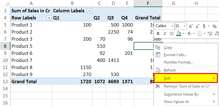
Whenever our mouse is on the "Sort" option, we can see another section where we select largest to smallest.

Example 2-8

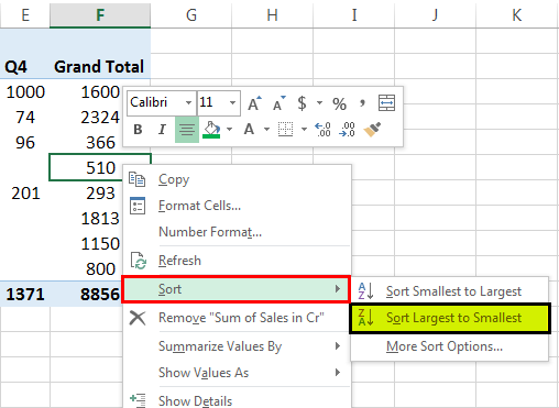
Now, we have sorted our data from largest to smallest in terms of sales in our PivotTable.

Example 2-9

Example #3

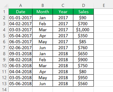
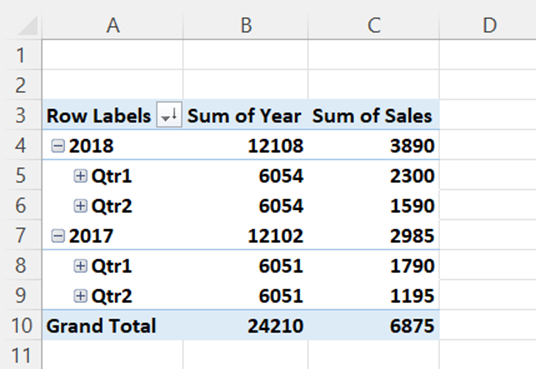
Consider the below table showing sales in years 2017 and 2018.

Pivot Table Sort - Example 3

Now, we have to create a pivot table by clicking on Insert - Tables - PivotTable.

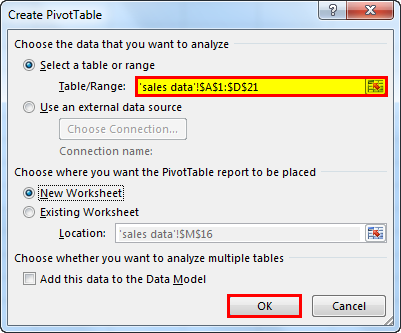
In the Create PivotTable window, we need to select the Table/Range: of the data we want to create a pivot table for. And then, click OK.

In the PivotTable fields, we need to select the sections which we want to view in our pivot table.

Now, right click on Row Labels more options and we can see Sort options, readily available.

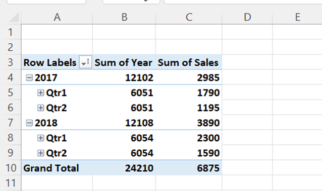
Let’s try both the options. If we sort from oldest to newest, the resulting pivot table appears as shown in the below image.

Example 3 - Pivot Table

If we sort from newest to oldest, the resulting pivot table appears as shown in the below image.

Example 3 - Pivot Table sort

Likewise, we can sort PivotTable in Excel.

Important Things To Note

Excel PivotTable Sort is done on a PivotTable. So, we must first generate a PivotTable.
Sorting depends on the data. It means if the data is numerical, it can be sorted from highest to smallest or vice versa.
If the data is in string format, it may be sorted in A to Z or Z to A.

Frequently Asked Questions

1. How to use pivot table sort by value?

Microsoft Excel allows you to sort data by a specific value, making it easier to analyze and understand your data. To sort by a specific value, follow these simple steps:

First, click on the arrow located next to Row Labels. This will open a drop-down menu.
2. From the drop-down menu, select "Sort by Value". This will sort all the values in the selected row by their respective values in ascending order.
3. If you want to sort by a specific column instead, click on the arrow next to Column Labels. Choose the desired field that you want to sort first, followed by the sort option you want.
4. In the "Sort by Value" box, you can select the value you want to sort from the "Select value" drop-down menu. This will sort the values based on the selected value.
5. Finally, choose the sort order you want from the "Sort options" menu. You can sort the values in ascending or descending order.
By following these steps, you can quickly sort your data by a specific value in Microsoft Excel.

2. How do you sort a PivotTable by sum?

To sort a column in descending order, follow these steps: first, click on the small drop-down arrow next to the "Labels" option. Then, select "More sort options" and check the "Descending" box. After that, choose the column you want to sort by from the drop-down menu. For example, you should sort by the sum of the total amount. Finally, click on "Apply" to sort the values in descending order. You can also sort values from lowest to highest using the same method.

3.How do I sort a pivot table by month?

To group the Dates column, right-click on any cell within it and select Group from the fly-out list. In the dialog box, choose Month. If you want to group only some of the list, you can specify the range of dates using the Starting at: and Ending at: fields.