Pivot Table Change Data Source

Last Updated :

21 Aug, 2024

Blog Author :

Edited by :

Reviewed by :

Table Of Contents

What Is Change Data Source For Pivot Table?

Pivot Table change data source option is used to change pivot table data when values in the original data are inserted or deleted. It is similar to updating the pivot table but is more advanced than just refreshing the data.

For example, consider the below pivot table showing products, sales and the grand total.

Pivot Table Change Data Source - Intro Example

Now, let us assume that the sales of product MNO and PQR has to be included in the pivot table.

We can simply click on PivotTable Analyze - Change Data Source.

The Change PivotTable Data Source window pops up. Here, change the cell range and click on OK.

We can see the data included in the pivot table.

Likewise, we can use change data source option in Excel.

However, in this article, we will show you how to change the data range for the PivotTable. Also, we will show you an automatic data range picker at the end of this article.

What Is Change Data Source For Pivot Table?

Pivot Table Change Data Source is an option used to update the already created pivot table.
Any changes, such as addition or deletion of values in the original data table in Excel worksheet can be reflected in the pivot table using change data source option.
To update, simply click on PivotTable Analyze > Change Data Source in Excel.
The Change PivotTable Data Source window opens up. We can simply select the new cell range and click OK to update pivot table.

How To Locate The Data Source Of Pivot Table?

One of the things is when we get the Excel workbook; sometimes, we may have a pivot table, We do not know exactly where the data source is.

Following are the steps to locate the data source of the PivotTable.

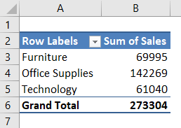
For example, look at the PivotTable below.
To identify the data source, place a cursor inside the PivotTable in any of the cells. It will open up two more tabs on the ribbon “PivotTable Analyze” and “Design.”
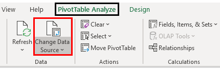
Go to “PivotTable Analyze” and click “Change Data Source.”
It will open up the below window. It will take you to the data worksheet with the data range selection.

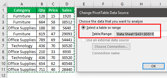
You can see that the data source is ‘Data Sheet’!$A$1:$D$11.In this, “Data Sheet” is the worksheet name, and “$A$1:$D$11” is the cell address. Like this, we can locate the data source range in Excel.

How To Change Data Source In Excel Pivot Table?

Below are some examples of changing the data source.

#1 – Change Data Source Of Pivot Table

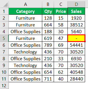
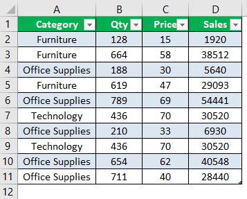
PivotTable has been created for the range of cells from A1 to D11 to reflect anything in this range in the PivotTable with the help of the “Refresh” button. So, for example, now we will change the sales number for the “Furniture” category.

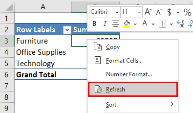
Go to the PivotTable sheet and right-click the “Refresh” option to update the PivotTable report.

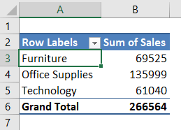
The “Furniture” category sales numbers will change from 69525 to 40432.

It is fine!!!

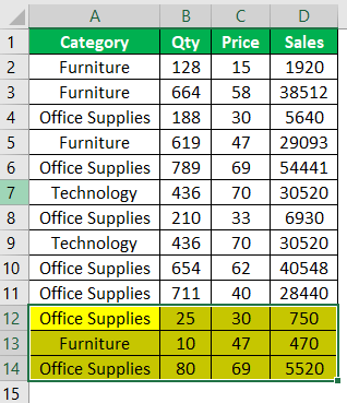
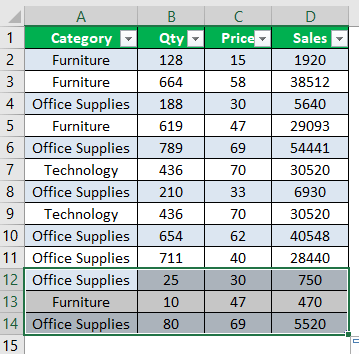
However, we have a problem: our data range selected for the PivotTable is A1:D11. So now, we will add 3 more data lines in rows from 12 to 14.

PivotTable “Refresh” will not work because the cell reference range given to the PivotTable is limited to A1:D11. So, we need to change the date range manually.

Go to “PivotTable Analyze” and click “Change Data Source.”

It will take you to the actual data sheet with the highlight of the already selected data range from A1:D11.

Now, delete the existing data range and choose the new data range.

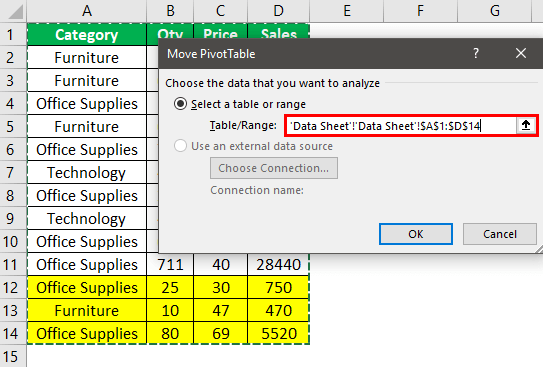
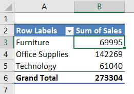
Click “OK,” and the PivotTable will show the updated data range result.

It looks fine. Assume that the data range scenario is increasing daily. If you have 10 to 20 PivotTables, we cannot go to each PivotTable and change the data source range, so we have a technique for this.

#2 – Auto Data Range Source Of Pivot Table

We cannot make the PivotTable with a normal data range and pick any additional data source. So, we need to make the data range for converting to Excel Tables.

Place a cursor inside the data cell and press Ctrl + T to open the “Create Table” window.

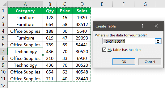
Ensure the “My table has headers” checkbox is ticked and click on “OK” to convert the data to the “Excel Table” format.

Usually, we select the data and then insert the PivotTable. But with Excel Table, we need to choose at least one cell in the Excel Table range and insert the PivotTable.

Now, add three lines of data just below the existing data table.

Return to the PivotTable and refresh the report to update the changes.

Such is the beauty of using Excel Tables as a data source for the PivotTable. It makes the data range selection automatic. We only need to refresh the PivotTable.

Important Things To Note

Excel Tables as the PivotTable makes the data range selection automatic. With a single ALT + A + R + A shortcut excel key we can refresh all the PivotTables.
We must press the shortcut key Ctrl + T to convert data to an Excel Table.

Frequently Asked Questions

1. What is pivot table change data source?

PivotTables are powerful and help us in analyzing the data. Before creating a PivotTable, we must select the data range we cover in the PivotTable report generation. Any deletion of data will affect if the refresh button is clicked. Likewise, any values that are changed will also affect the refresh button.

However, one of the complaints of the PivotTable users is that any additional data beyond the data range selection will not impact the PivotTable report. It is also one of the problems because whenever there is extra data, we need to change the data range. In such cases, we use change data source option.

2. Explain how to use pivot table change data source with an example.

For example, consider the below pivot table showing products, sales and the grand total.

FAQ 2.jpg

Now, let us assume that the sales of products E, and F has to be included in the pivot table.

We can simply click on PivotTable Analyze - Change Data Source.

The Change PivotTable Data Source window pops up. Here, change the cell range and click on OK.

FAQ 2 - Output

We can see the data included in the pivot table.

Likewise, we can use change data source option in Excel.

3. What is an alternative method to update pivot table?

We can simply change the data in the original table and then, right click anywhere on the pivot table. Next, click on Refresh button. This will immediately update the pivot table.