Pivot Table Group by Month

What Is Pivot Table Group By Month?

Pivot table group by month is used to group or summarize data based on dates. This helps users to calculate the total for each month as it automatically gives the total and saves users’ time as we don’t have to count daily transactions.

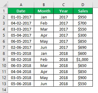
For example, consider the below table showing sales in different months in the year 2017 and 2018.

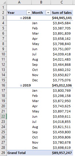
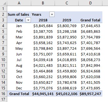
Now, using pivot table group by dates option, we can calculate the grand total in 2017 and 2018 as shown in the below image.

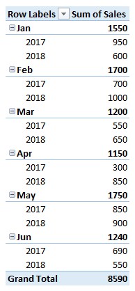
As shown in the image, we can see the sum of sales month-wise and the grand total.

Table of contents

• What Is Pivot Table Group By Month?
  • How To Use Pivot Table Group By Month?
  • Examples
  • Important Things To Note
  • Frequently Asked Questions
  • Recommended Articles
• Pivot table group by month is an option used to find the total of data based on month in Excel.
• This method helps users calculate the total for each month and also, summarizes the total sales. We can view the result in the pivot table.
• The month can be calculated by using the formula =TEXT(value,format_text)
• Similarly, year can be calculated using the formula =YEAR(serial_number)
• Click on Design > Report Layout > Show in outline form to obtain the result in outline form.

How To Use Pivot Table Group By Month?

We can group data by month using pivot table. This will help users calculate the total without any difficulty.

Let’s learn how to use pivot table group by month using the below examples.

Examples

Example #1 - Group Dates By Months

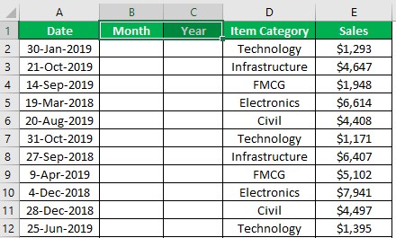
To demonstrate this example, we have prepared sample data you can download to practice with us.

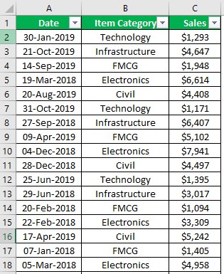
This data is for two years, 2018 and 2019, daily. We need to summarize this data to get monthly sales values, so we need to extract month and year from the dates to analyze the sales on a monthly and yearly basis.

First, insert the PivotTable and apply the PivotTable, as shown below.

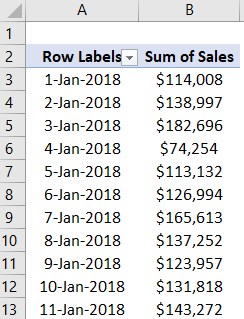
It has given us a daily summary report to arrive at month and year in two ways. First, we will see how to add months and years from the date column.

Insert two more columns and name them “Month” and “Year,” respectively.

For the “Month” column, insert the below formula.

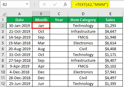
This TEXT function takes the reference of the date column and applies the format as a short month name with code “MMM.”

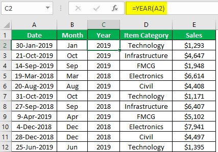
Now, apply the below formula to extract YEAR from the “Date” column.

Next, insert a PivotTable by selecting the data.

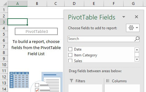
Now, drag and drop the “Year” and “Month” columns to the “ROWS” area and the “Sales” column to the “VALUES” area. We will have a PivotTable like the one below.

Change the report layout to the “Outline” form.

Now, our report looks like the one below.

Looks good. This technique is followed by users who do not know about the grouping technique in a PivotTable. We will see this now.

This topic opens up many avenues for further exploration. If you’re intrigued by these concepts, this Excel Pivot Tables Crash Course might provide additional insights and hands-on experience.

Example #2 - Group Dates In The Pivot Table

Inserting two extra columns to add month and year looks like an additional task. Now, imagine the scenario where we need to see a quarterly summary, so we need to add another column and use a complex formula to arrive at the quarter number.

So, it looks tedious to do all of these tasks. However, we can only group the dates in pivot tables without adding extra columns.

Follow the below steps to group PivotTables by dates.

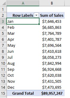
1. Insert the PivotTable first, like the one below.

   
   

2. Right-click on any of the cells of the “Date” column and choose the “Group” option.

   
   

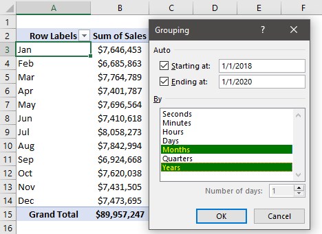
3. When you click on the “Group” option, it will show us below the window.

   
   
   
   In this window, it has picked automatic dates starting at and ending at dates.

4. Choose the “Group By” option as “Months” and click on “OK” to group the dates by “Months.” And you will see the PivotTable result below.

   
   

The problem here is we have two years of data. Since we have grouped by “Month,” it has grouped by months and did not consider years while choosing the grouping option to select both “Month” and “Year.”

Click on “OK.” We will have a new PivotTable like the one below.

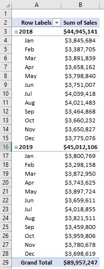
It is exactly similar to the previous manual method we have followed.

So using PivotTable dates, only we can group the dates according to the months, years, and quarters.

We need to notice that we had only “Date” as the “ROWS” area column. But after grouping, we can see another field in the “ROWS” area section.

Because we have used the years as the second grouping criteria, we can see “Years” as the new field column, so instead of seeing the long PivotTable, drag and drop the “Years” field from the “ROWS” area to the “COLUMNS” area.

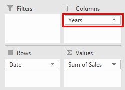
So now, we can easily look at and read the PivotTable report.

Important Things To Note

• We can group dates and time values in Excel.
• We must choose the kind of group we are doing.
• To group, click on the pivot table and choose Group.

Frequently Asked Questions

1. What is pivot table group by month?

In any sector, data is captured daily, so when we need to analyze the data, we use PivotTables. So, it will also summarize all the dates and give them daily. But who will sit and see everyday transactions? Rather, they want to see the overall monthly total, which comprises all the dates in the month and gives the single total for each month so that we will have a maximum of 12 lines for each year. So, using Pivot Table in Excel, a grouping of dates into months is possible.

2. Explain the use of pivot table group by month with an example.

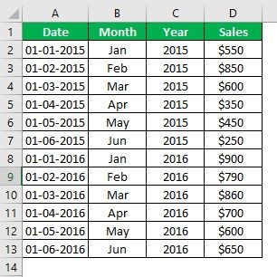
Consider the below table showing sales in different months in the year 2015 and 2016.



Now, using pivot table group by dates option, we can calculate the grand total in 2015 and 2016 as shown in the below image.


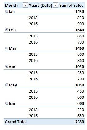
As shown in the image, we can see the sum of sales month-wise and the grand total.

3. How to find month and year in the data?

Consider the data has two columns – date and sales. To find the month and year, we can simply use the formulas – TEXT and YEAR.

• The syntax of TEXT is =TEXT(value,format_text)
• The syntax of YEAR is =YEAR(serial_number)

Recommended Articles

This article is a guide to PivotTable Group by Month. Here, we discuss how to group dates by months in a PivotTable with some examples. You may learn more about Excel from the following articles:

• Pivot Table Add Column
• Using VLOOKUP in Pivot Table
• Examples of Pivot Table
• VBA Pivot Table
• Barcode in Excel