How to Refresh Pivot Table in Excel? (Using Top 4 Methods)

How to Refresh Pivot Table in Excel?

Below are the top 4 methods to refresh the Pivot Table in Excel

Refresh Pivot Table By Changing Data Source
Refresh Pivot Table using Right Click Option
Auto Refresh Pivot Table Using VBA Code
Refresh Pivot Table When you open the Workbook

Now let us discuss each method in detail with an example –

#1 Changing the Data Source Refresh Pivot Table

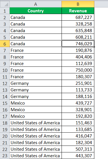
Step 1: I have sales data from different countries.

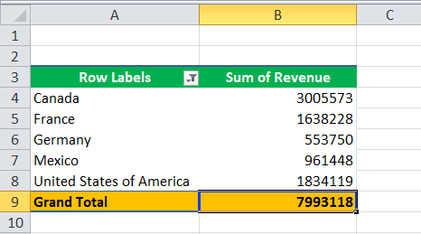
Step 2: Let me apply the pivot table to this data.

Step 3: Now I am going back to my pivot table data and adding a few more data to the table.

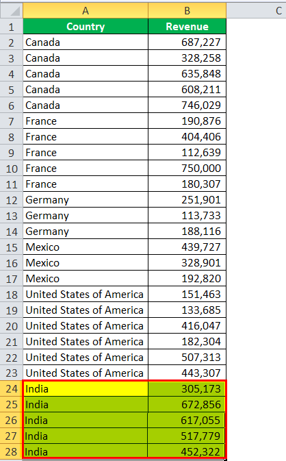
I have added five lines of the data. If I go and see the table, it is not showing the updated values.

Let me audit what is the range of the pivot table data.

Step 4: Select the pivot table and go to Options and Change Data Source.

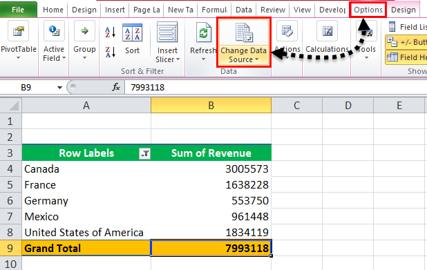
Step 5: Once you click on Change Data Source this will take you to the datasheet along with the below box.

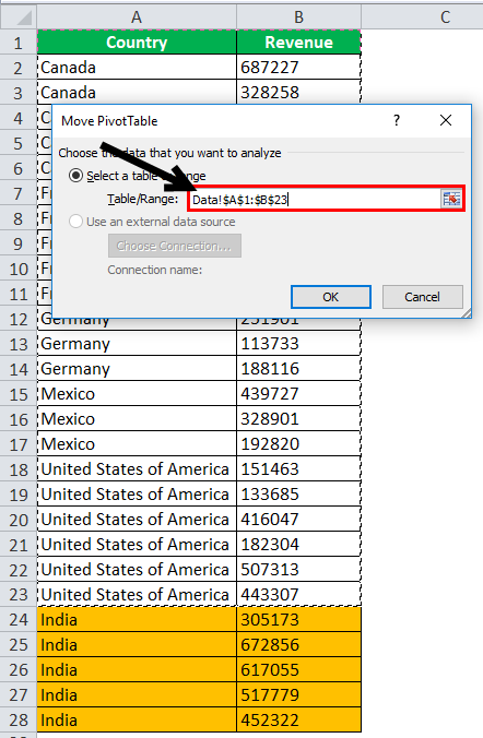
Look at the range it has. It has the data range from A1 to B23, whereas my data is there from A1 to B28.

Popular Course in this category

All in One Excel VBA Bundle (35 Courses with Projects)4.9 (1,353 ratings) 35+ Courses | 120+ Hours | Full Lifetime Access | Certificate of Completion

View Course

Step 6: In the same dialogue box, change the source data from A1 to B23 to A1 to B28.

Step 7: Now click on OK it will add the new data to the pivot table and refresh it.

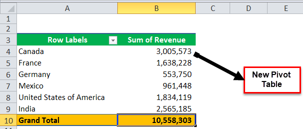
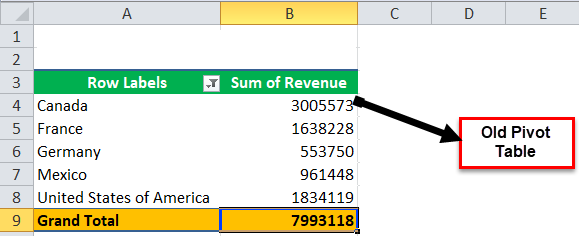
#2 Right Click on the Pivot Table and Refresh Pivot Table Excel

I am taking the previous data as an example.

Step 1: Here I am not adding any amount of data to the list rather I am just changing the existing numbers.

Step 2: Here on cell B10, I have to change the value from 677434 to 750000. If I go to the pivot table still it is showing the old values for the country France.

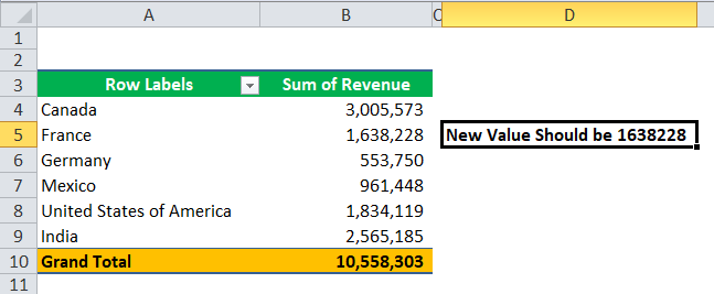
Step 3: The new value for the country France supposed to be 1638228 but it is showing the old value only. We need to do one simple thing here. Right-click on the Refresh.

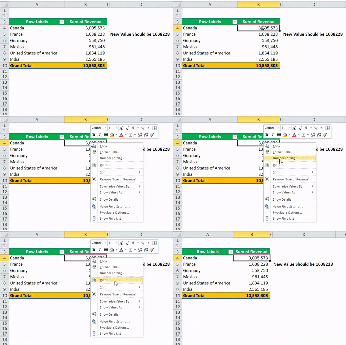
Step 4: Click on the Refresh button to update the new values.

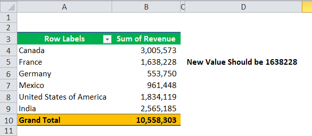
Okay, now our Pivot Table is showing updated values.

Now the question is if I have 10-pivot tables can I update each one of them going to each pivot table and update.

We have the shortcut to refresh all the pivot tables in excel one single shot. Below is the shortcut key to refresh all the pivot tables once.

We can find this option under the Data tab.

#3 Using Auto Refresh Pivot Table Excel VBA Code

Ok, we know how to refresh the pivot table to new values. Whenever we change the values we every time we need to update manually.

If the data changes frequently and updating each and every pivot table is not that easy. We are humans and we tend to forget at times.

To come off that danger we have a VBA code, which can update or refresh as soon as there are any changes.

Follow this section of the article to learn the VBA code that refreshes the pivot table in excel automatically.

Step 1: Go to the Developer tab and click on Visual Basic.

Step 2: Click on Visual Basic. Go to This Workbook and double click on that.

Step 3: From the dropdown list select Workbook.

Step 4: Once you have selected the workbook it will automatically create one macro for you. Ignore that.

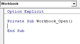
Step 5: From the Right-hand side drop-down select Sheet Change. It will insert one more macro for you.

Step 6: Now copy and paste the below code the macro that has created for the second time.

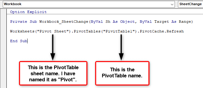
What this code will do is if there is any change in the sheet it will refresh the pivot table in excel automatically for you.
Note: Once you copy and paste the code, you have to save the workbook as Macro-Enabled Workbook.

#4 Refresh Pivot Table When you Open the Workbook

We can refresh the pivot table while opening the workbook.

Right Click on any of the pivot table and select Pivot Table in Excel option

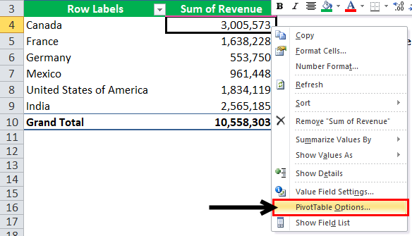
Click on this option

Go to Data and check Refresh Data when opening the file.

This will refresh the pivot table in excel whenever you open the excel file.

Things to Remember

You can choose any of the above methods to refresh your pivot tables.
In the case of VBA code you, need to save your workbook as the macro-enabled workbook.
The easiest for me to refresh is the shortcut ALT + A + R +A
You can rename your pivot table under pivot options.
In VBA code, you need to mention each of the pivot table names in the case of multiple pivot tables.