Row Header In Excel

Last Updated :

21 Aug, 2024

Blog Author :

Edited by :

Reviewed by :

Table Of Contents

What Is Excel Row Header?

The ROW Header in Excel is one of the main components in Excel worksheet features. It gives an idea of which cell we are working on, such as which row and column number cell.

We may find it difficult to print the Excel Row header in a large dataset or lose them when scrolling from left to right. We can use options such as show/hide, freeze, and lock to print them.

For example, we can see the Row Headers in Excel in the image below.

Row Header in Excel

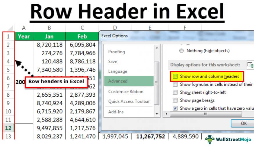
Table of contents

What Is Excel Row Header?
The Row Header in Excel helps the user to immediately identify the cell address of the active cell.
The Rows and Columns are the main features that create a worksheet. They run horizontally from top to bottom and vertically from left to right, giving the tabular format to the sheet. And when a Row and Column intersect, they form a Cell.
In a workbook, we can insert, delete, hide, resize, move, copy, and group Rows and Columns. Any changes we make apply only to the current worksheet.
The shortcut key for hiding or showing Row and Column headers is ALT + W + V + H.
We cannot show/hide headers for the entire workbook at once, however, we can select multiple worksheets and show/hide headers.

How To Show Or Hide Row Headers In Excel?

We will consider the following example of a worksheet to show or hide Row Header In Excel.

We can see all the row and column headers in excel, by default.

Row Headers Example 1

The procedure to show/hide the Row and Column header is as follows:

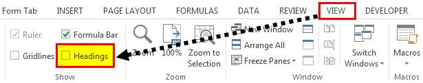
First, select the “VIEW” tab - go to the “Show” group - uncheck the “Headings” option checkbox to hide them, and check/tick the checkbox to show them in the current sheet, as shown below.

Row Headers Example 1-1

The Output is shown below:

Row Headers Example 1-6

How To Freeze And Lock Row Headers In Excel?

We will consider the following example of a worksheet to freeze and lock Row Header In Excel.

Now, take a look at the huge datasheet below.

Row Headers Example 2

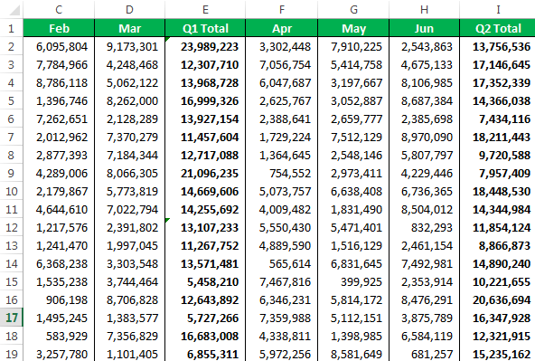
The first column is the heading for all the rows for this data. Now, we will move from left to right. When we move from left to right to the end of the dataset or the last column of the data, we cannot see the row headers now.

Row Headers Example 2-1

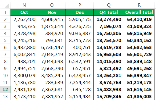
We can only see Excel row headers but not the data row headers. It is so confusing which row header we are referring to now. Going back and seeing the row header now and then is a frustrating job to do.

The steps to lock and freeze our row heading are as follows:

Step 1: Go to View - Freeze Panes.

Go to View > Freeze Panes

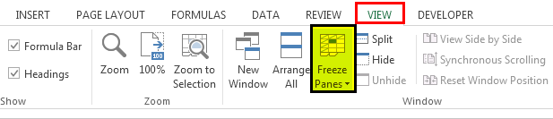
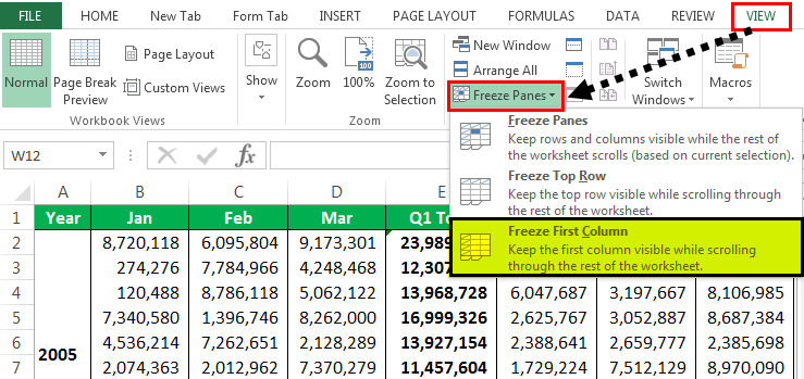
Step 2: Click the Freeze Panes option drop-down, and select the “Freeze First column”.

drop-down list of Freeze Panes

Step 3: It does not matter where we are on the sheet. We can see our row header at all points in time as it is locked and frozen in the dataset.

Row Headers Example 2-5

Now, it is easier to understand exactly which row we are referring to and what the row header is.

Using row headers can help with data identification, organization, and navigation. To know about other Excel features that can improve the appeal of a report, one can take the help of this Excel for Finance Course.

How To Print Excel Row & Column Headers?

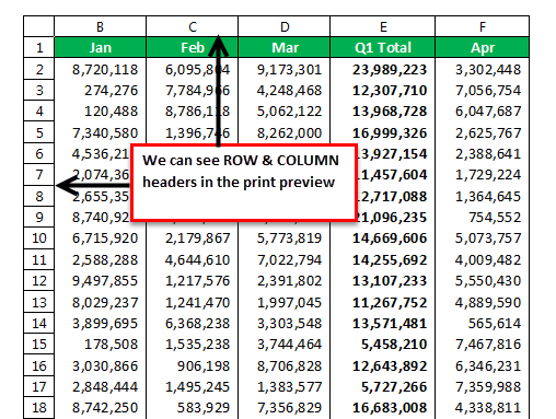
We often do not worry about printing our Row and Column headers in our printing options. But now, look at the screenshot below of the print preview in excel.

Row Headers Example 3.1

It shows only the data range but not our Excel Row and Column headers. Remember, “Data Headers” are user headers, and Row and Column headers are Excel headers.

To print the Row and Column headers, we need some twists in the print settings before we go ahead and print. The steps are,

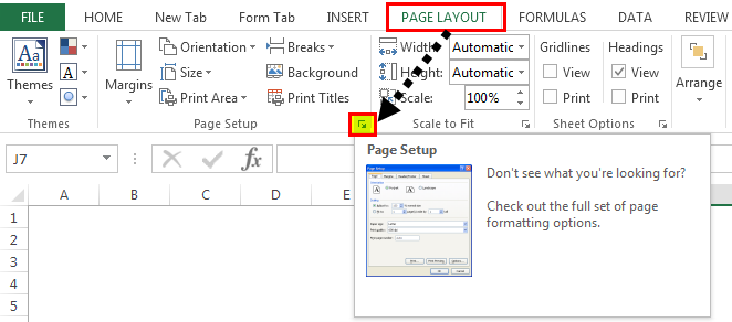
Step 1: Go to “PAGE LAYOUT”, and click the “PAGE SETUP” arrow.

Page Layout - Page Setup

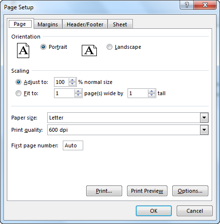
Step 2: Now, we will see the Page Setup window.

Page Setup Window

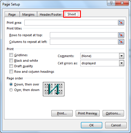
Step 3: Click the “Sheet” tab in this “Page Setup” window.

Row Headers Example 3-2

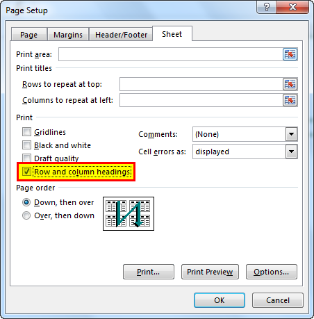
Step 4: Under this tab, check/tick the “Row and column headings” checkbox, and click “OK”, as shown below.

Row Headers Example 3-3

Step 5: Now, see the print preview. We can see row & column headers here.

Row Headers Example 3-4

Important Things To Note

Ensure never to Hide the Row and Column headers when dealing with a huge dataset, as it will only add confusion.
We can freeze or lock as many rows as possible by placing the cursor after the last row.

Frequently Asked Questions

1. How can we Show or Hide the Row Header in Excel using the Excel Options?

Another way to Show or Hide the Row and Column headers are as follows:
1. Go to the “FILE” tab - click the “Options” from the list, as shown below.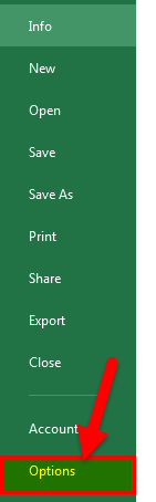

Go to FILE u0026 Options

2. The “Excel Options” window opens.
• On the left, select the “Advanced” option.
• On the right, scroll down to the “Display options for this worksheet” option, check/tick the “Show row and column headers” check box to Show the headers, and uncheck the option to Hide them.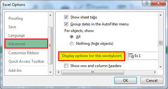

Display option for this worksheet

3. Uncheck the box “Show Row and Column headers.”

Show row u0026 column headers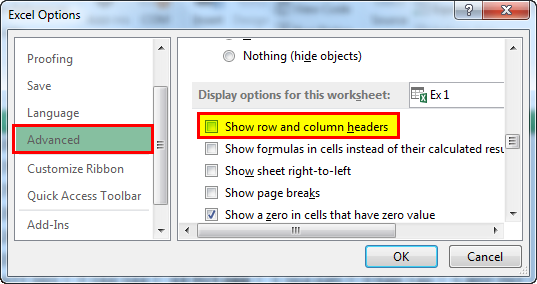

4. It will hide Row and Column headers from the selected worksheet.

2. Name few other features or components in Excel, like Row and Column headers.

A few features or components in Excel are as follows:
#1 – Rows of Excel - Excel contains a fixed number of rows, 1048576, with the row numbers displayed on the left side of the worksheet. The Name Box displays the active cells cell address, the digit in the address indicates the cell’s row number, as shown below.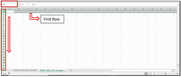

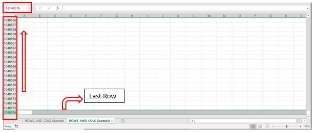
Row Header in Excel - First Row

Last Row

Furthermore, as the rows run horizontally across the worksheet from top to bottom, we scroll up and down to navigate from one row to the other using the Vertical Scroll Bar.

#2 – Columns of Excel - Excel contains a fixed number of columns, 16384. The column names A to XFD appear on the top of the worksheet. The Name Box displays an active cells cell address, the alphabets in the address indicate the cell’s column name, as shown below.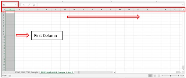

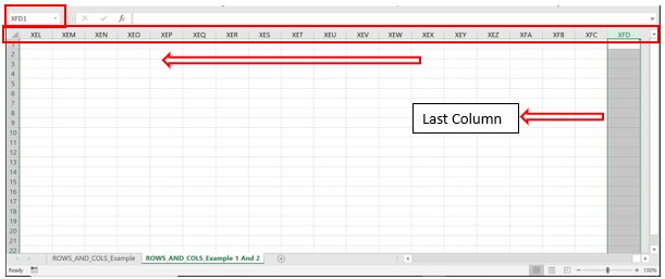
Row Header in Excel - First Column.jpg

Last Column

Furthermore, as the columns run vertically across the worksheet from left to right, we scroll left and right to navigate from one column to the other using the Horizontal Scroll Bar.

#3 - Cell of Excel - The intersection of a row and column forms a Cell. A cell has an address to locate it in a worksheet. The address is a combination of the name and number of the column and row that intersect to form the specific cell.
For example, the image below shows column C and row 5 intersecting to form cell C5.
We can enter the cell address in the Name Box on the top-left corner of the worksheet, and press Enter to select the specific cell. Otherwise, we can scroll the worksheet, and click on the required cell to select it.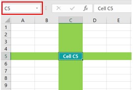

Row Header in Excel - Cell of Excel

3. What are the uses of Row Header in Excel?

A few uses of the Row Header in Excel are,
• We are able to print the worksheet with the Row Headers for clear understanding.
• Irrespective of the cells selected, we can easily identify the cell address when we have the Row Headers.