Project Timeline In Excel

Last Updated :

21 Aug, 2024

Blog Author :

Edited by :

Reviewed by :

Table Of Contents

What Is Project Timeline In Excel?

A project timeline is the list of tasks recorded to be accomplished to finish the project within the given period. In simple words, it is nothing but the project schedule/timetable. All the tasks listed will have a start date, duration, and end date so that it becomes easy to track the project’s status and complete it within the given timeline.

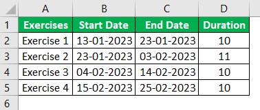
For example, the below table shows the list of exercises in column A and the number of days required to complete in columns, B and C. Similarly, we also have the duration required to complete each exercise in column D. Now, let us learn how to create project timeline in excel.

The steps used to create project timeline in excel are:

Step 1: Go to the Insert tab.

Step 2: Click on the drop-down list of Insert Column or Bar Chart from the Charts group and select 2-D Bar from the available types.

We can see 2-D stacked bar in our worksheet.

Step 3: Right-click on the chart and choose Select Data.

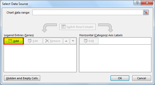
Step 4: The Select Data Source window pops up. Click on the Add button.

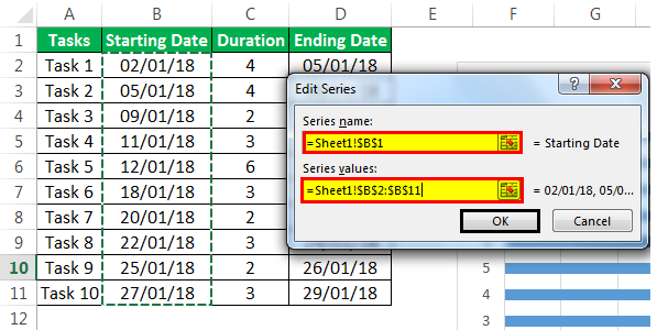
Step 5: The Edit Series window appears.

Choose the Series Name: and Series Values: and click OK.

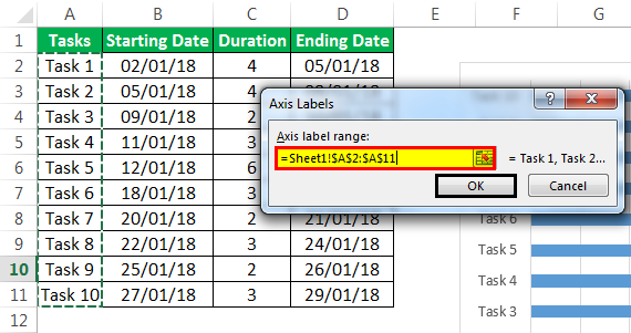
Step 6: The Select Data Source window pops up. Select the Start Date and then click on the Edit button.

Step 7: The Axis Labels window pops up. Enter the values in the Axis label range: dialog box.

Click OK twice to obtain the chart.

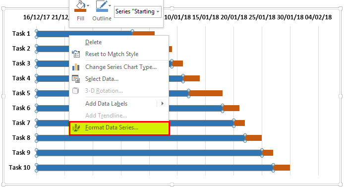
Step 8: Right-click on the blue bars and choose Format Data Series.

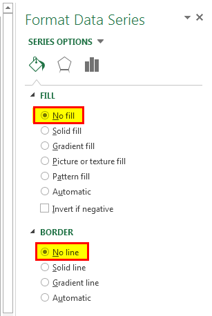
Step 9: The Format Data Series tab appears on the right side of the Excel sheet.

Click on the No Fill and No Line options.

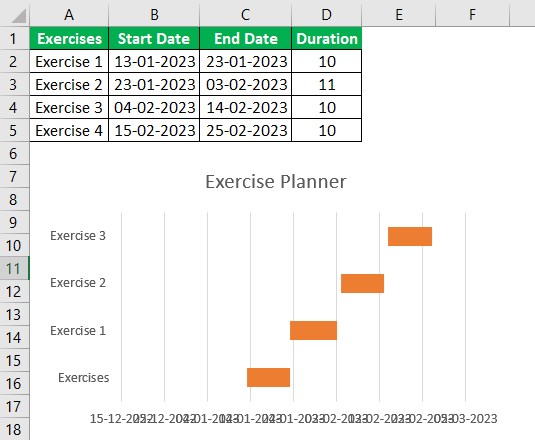
We have now created our project timeline in Excel.

What Is Project Timeline In Excel?

The project timeline in excel is a Stacked Column Graph representing the Excel project timeline in horizontal bars.
It is also called as Gantt chart.
The horizontal bars indicate the duration of the task/activity of the project timeline in Excel.
Project timeline in Excel reflects the addition or deletion of any activity within the source range, or the source data can be adjusted by extending the range of rows.
This chart does not provide detailed information about the project and lacks real-time monitoring ability.

How To Create A Project Timeline In Excel? (With Steps)

We can create project timeline in Excel or Gantt charts manually or use Microsoft’s template.

While opening Excel worksheet, search for Gantt Project Planner to create a project timeline in Excel.
Next, click on Gantt project planner > Create in the pop-up window.

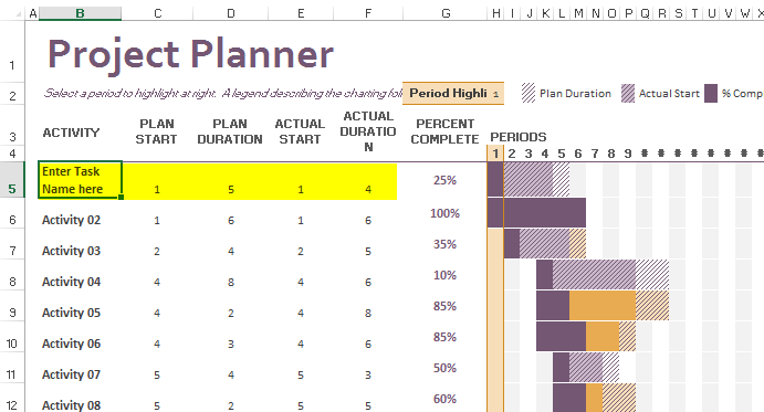
Now, we can use the template to enter our project details.

Similarly, let us have a look at the following examples to understand how to create project timeline in Excel.

Examples

Example #1

Creating a Gantt chart using a normal stacked bar graph:

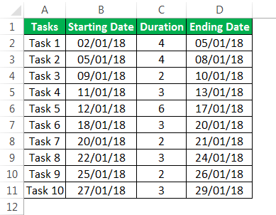
List down the tasks/activities that need to be completed in the Excel sheet (as shown below).
Enter the start date for each task in the column next to the activities.
Update the task’s “Duration” next to the “Starting Date” column (duration is the number of days required for the particular task/activity to be completed).
We can insert the “Ending Date” for the activities next to the “Duration” column. This column is optional because this is just for reference and will not be used in the chart.

Note: We can insert duration directly or use a formula to determine duration.

The above table calculates duration using the formula: Ending Date (-) Starting Date.

In the formula, “+1” is used to include the day of the starting date.

Now, let us begin to build a chart.

In the ribbon, go to the “INSERT” tab and select the “Bar graph” option in the “Charts” sub-tab. Next, choose the “Stacked” bar (the second option in the “2-D Bar“ section).

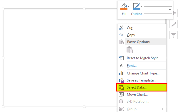
By selecting this graph, a blank chart area may appear. Select that empty area and right-click to choose the “Select Data” option.

“The “Select Data Source” window may appear to select the data. Next, click on the “Add” button under “Legend Entries (Series).”

When the “Edit Series” pop-up appears, select the “Starting Date” label as the “Series name.” In this example, cell B1. Also, choose the list of dates in the “Series values” field. Then, press the “OK” button.

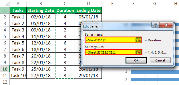
Again, press the “Add” button to select the “Series name” and values of the “Duration” column the same as above.

After adding both the “Starting Date” and “Duration” data into the chart,

Click on “Edit” under the “Horizontal (Category) Axis Labels” on the right-hand side of the “Select Data Source” window.

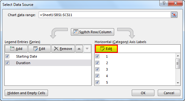
In the “Axis Labels” range, select the list of tasks starting from “Task 1” to the end and click on “OK.”

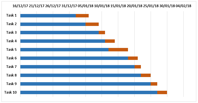
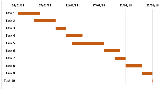
Below is the output we can see after completing all the above steps.

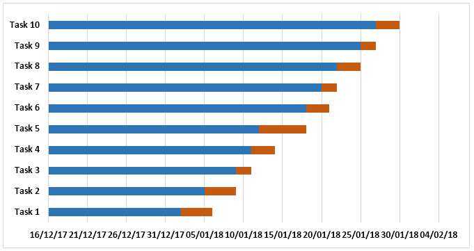
The above chart shows the list of tasks on the Y-axis and dates on the X-axis. But, the list of tasks shown in the chart is in reverse order.

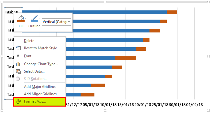
To change this:

We must select the axis data and right-click to select “Format Axis.”

In a “Format Axis” panel, under the “Axis Options” section, check the “Categories in reverse order” box.

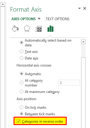
When the categories are reversed, we may see the chart below.

We need to make a blue bar invisible to show only the orange bars, which indicate the duration.

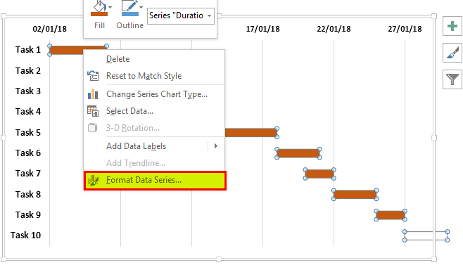
Click on the blue bar to select and right-click “Format Data Series.”

In the “Format Data Series” panel, select “No Fill” under the “Fill” section and “No line” under the “Border” section.

The chart looks as below.

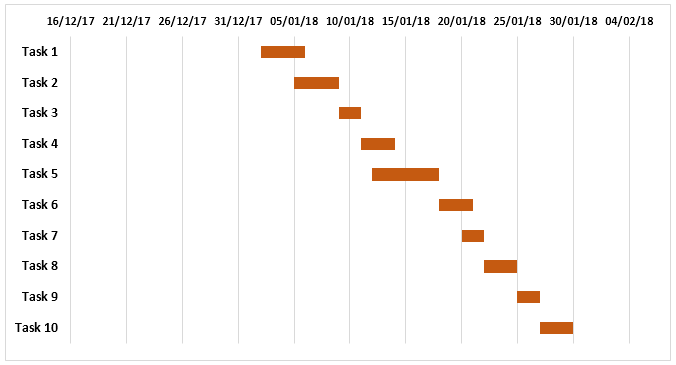
Now, the project timeline Excel Gantt chart is almost completed.

Remove the white space at the beginning of the chart.

Right-click on the date given for the first task in a table and select “Format Cells.”

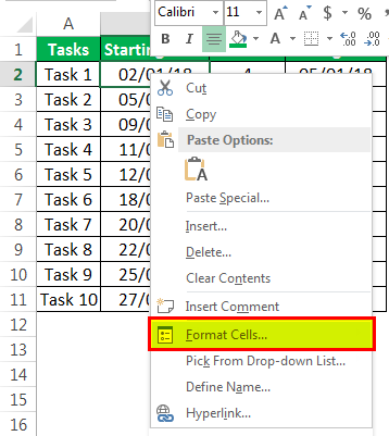
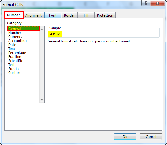
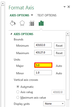
Note the number in the window under the “Number tab” and “General” categories.

(In this example, it is 43102)

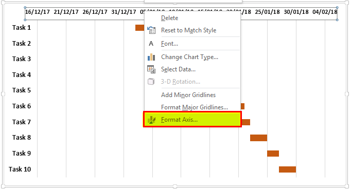
Click on the dates on the top of the chart and right-click, select “Format Axis.”

In the panel, change the "Minimum" number under the "Bounds" options to the number you have noted.

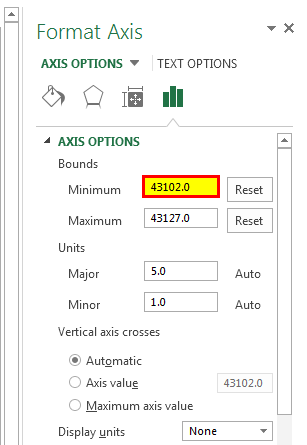
The units of date can adjust the scale as you want to see in the chart. (in this example, we have considered “Units” as 5)

The chart may look like the one given below.

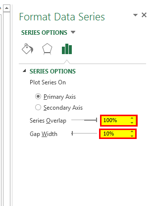
Trim the chart to make it look nicer by eliminating the white space between the bars.

Click on the bar anywhere. Then, right-click and select “Format Data Series.”

Keep the “Series Overlap” at 100% and adjust the “Gap Width” to 10% under the “Plot Series On” section.

We can add the data labels to the bars by selecting “Add Data Labels” using right-click.

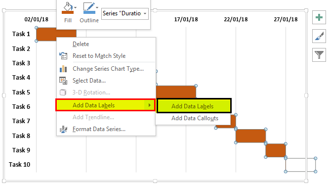
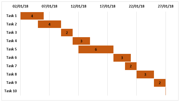
The data labels are added to the charts.

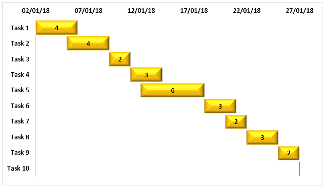
We can apply 3-D format to the chart to give some effects by removing the gridlines, and the color of the bar and font can be changed as required in the “Format Data Series” panel.
We can show the dates horizontally by changing the text alignment if required to show all dates.

Ultimately, the project timeline Gantt chart in Excel may look like this.

Example #2

Creating a Gantt chart using the project timeline template available in Excel:

Gantt charts can be created using Microsoft’s template readily available in Excel.

Click on the “Start” button and select “Excel” to have a new Excel sheet opened.
While opening, it shows the options to choose from. Search for “Gantt Project Planner to create a project timeline in Excel.

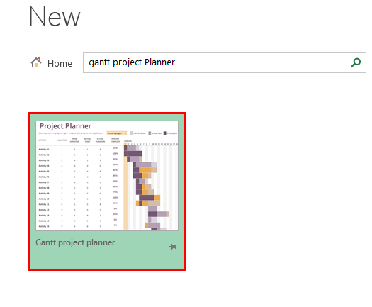
Click on “Gantt project planner” and click on “Create” in the pop-up window.

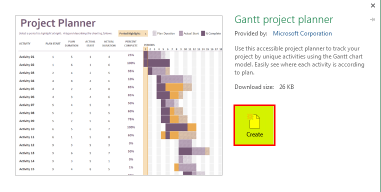
The template is ready to start by entering your project details in the given column per the headers and seeing the bars reflecting the timeline.

Important Things To Note

While using project timeline in Excel, we need to find the duration of the tasks.
The formula used to find duration is =End Date – Start Date
The #VALUE! Error occurs when the dates are not in correct format.

Frequently Asked Questions

1. What is project timeline in Excel?

A project timeline is one of the important aspects of project management. It is required to plan and determine the flow of tasks from the beginning to the end of the project.

2. How project timeline in Excel is represented?

The easiest way of representing the project timeline in Excel is through graphical representation. It can be created using the charts in Excel. It is called the “Gantt Chart.” Gantt chart (named after its inventor Henry Laurence Gantt) is one of the Bar Charts in Excel and a popular tool used in project management, which helps visualize the project schedule.

3. Explain how to use project timeline in Excel with an example.

The below table shows the list of assignments in column A and the number of days required to complete in columns, B and C. Similarly, we also have the duration required to complete each exercise in column D. Now, let us learn how to create project timeline in excel.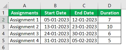

Project Timeline in Excel - FAQ 3

The steps used to create project timeline in excel are:

Step 1: Go to the Insert tab.
Step 2: Click on the drop-down list of Insert Column or Bar Chart from the Charts group and select 2-D Bar from the available types.
We can see 2-D stacked bar in our worksheet.
Step 3: Right-click on the chart and choose Select Data.
Step 4: The Select Data Source window pops up. Click on the Add button.
Step 5: The Edit Series window appears.
Choose the Series Name: and Series Values: and click OK.
Step 6: The Select Data Source window pops up. Select the Start Date and then click on the Edit button.
Step 7: The Axis Labels window pops up. Enter the values in the Axis label range: dialog box.
Click OK twice to obtain the chart.
Step 8: Right-click on the blue bars and choose Format Data Series.
Step 9: The Format Data Series tab appears on the right side of the Excel sheet.
Click on the No Fill and No Line options.

We have now created our project timeline in Excel.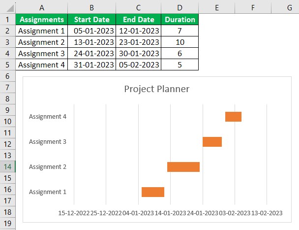

Project Timeline in Excel - FAQ 3 - Graph

Likewise, we can use project timeline in Excel with chart title.