Advanced Excel Formulas

Last Updated :

Blog Author :

Edited by :

Reviewed by :

Table Of Contents

What Are Advanced Excel Formulas?

Advanced Excel Formulas are the formulas that are not so commonly used. These are inbuilt formulas in Excel that are used to retrieve specific datafrom an existing dataset which might be like duplicating the data, filtering w.r.t specific criterias, conditional formulas, etc. These functions are used to generate reports, create dashboards, etc.

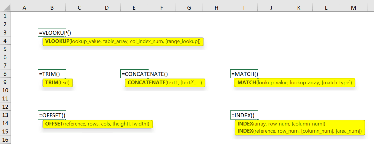
For example, a few of the inbuilt Advanced Excel formulas are given in the image below.

What Are Advanced Excel Formulas?

The Advanced Excel Formulas help us understand the inbuilt advanced formulas used for generating reports for concerns, companies, etc.
In Excel, VLOOKUP is the most commonly used LOOKUP function. Another important lookup function is HLOOKUP and XLOOKUP. Therefore, V stands for vertical lookup in VLOOKUP, and H stands for horizontal lookup in HLOOKUP.
In VLOOKUP, we cannot have a primary column on the right of the column for which we want to populate the value from another table.
One can combine INDEX and MATCH to overcome the limitation of VLOOKUP.
We can use the OR function instead of AND to satisfy one of the many conditions.

List Of Top 10 Advanced Excel Formulas & Functions

The Top 10 Advanced Excel Formulas & Functions we will consider in this article are as follows:

VLOOKUP Formula in Excel
INDEX Formula in Excel
MATCH Formula in Excel
IF AND Formula in Excel
IF OR Formula in Excel
SUMIF Formula in Excel
CONCATENATE Formula in Excel
LEFT, MID, and RIGHT Formula in Excel
OFFSET Formula in Excel
TRIM Formula in Excel

#1 - VLOOKUP Formula in Excel

It is one of the most used formulae in Excel mainly due to the simplicity of this formula and its application in looking up a certain value from other tables, which has one standard variable across these tables.

For example, if we have two tables detailing a company’s employee salary and name, with “Employee ID” being a primary column, and we want to get the salary from Table B in Table A.

We can use VLOOKUP as below.

It will result in the table below when we apply this advanced Excel formula in other cells of the “Employee Salary” column.

Drag the formula to the rest of the cells.

There are three major delimitations of VLOOKUP:

We cannot have a primary column on the right of the column for which we want to populate the value from another table. The “Employee Salary” column cannot be before the “Employee ID.”
In the duplicated values in the primary column in Table B, the first value will get populated in the cell.
If we insert a new column in the database (e.g., insert a new column before “Employee Salary” in Table B), the output of the formula could be different based on the position that we have mentioned in the formula (in the above case, the result would be blank).

#2 - INDEX Formula in Excel

It is used to get the value of a cell in a given table by specifying the number of rows, columns, or both. E.g., to get an employee’s name at the 5th observation. Below is the data.

We can use the advanced Excel formula below:

We can use the same INDEX formula in getting values along the row. So, for example, when using both row and column numbers, the syntax would look like this:

The above formula would return as “Rajesh Ved.”

Note: If we insert another row into the 5th row, the formula will return as “Chandan Kale.” Hence, the output would depend on any changes in the data table over time.

#3 - MATCH Formula in Excel

It returns the row or column number when a specific string or number is in the given range.

In the below example, we are trying to find “Rajesh Ved” in the “Employee Name” column.

The formula would be as given below:

The MATCH function would return 5 as the value.

The 3^rd argument is used for the exact MATCH. We can also use +1 and -1 based on our requirements.

#4 - IF AND Formula in Excel

There are many instances when one needs to create flags based on some constraints. We all are familiar with the basic syntax of IF. We use this advanced excel IF function to create a new field based on some existing field constraints. But what if we need to consider multiple columns while creating a flag?

E.g., in the below case, we want to flag all the employees whose salary is greater than 50,000. But “Employee ID” is greater than 3.

We would use the IF AND formula in such cases. Please find below the screenshot for the same.

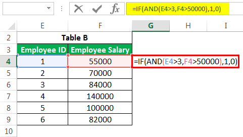
It would return the result as 0.

We can have many conditions or constraints to create a flag based on multiple columns using AND.

#5 - IF OR Formula in Excel

Similarly, we can use the OR function in Excel instead of AND if we need to satisfy one of the many conditions.

If any condition is satisfied in the above cases, we will have the cell populated as 1, else 0. We can substitute 1 or 0 with some substrings with double quotes (“”).

#6 - SUMIF Formula in Excel

The advanced Excel SUMIF function in excel

filters the required data based on certain criteria or condition and finds the sum of the returned numeric values.

E.g., We can find the total salaries of the employees whose employee IDs fall under a specific criterion, say greater than three.

Let us enter the SUMIFS formula:

The formula returns the results as 322000.

We can also count the number of employees in the organization having an employee ID greater than 3 using COUNTIF instead of SUMIF.

#7 - CONCATENATE Formula in Excel

It is one of the formulas used with multiple variants, which helps us join several text strings into one text string.

For example, if we want to show “Employee ID” and “Employee Name” in a single column.

We can use this CONCATENATE formula here.

The above formula will result in “1Aman Gupta”.

We can have one more variant by putting a single hyphen between ID and NAME. E.g., CONCATENATE(B3,”-“,C3) will result in “1-Aman Gupta”. We can also use this in VLOOKUP when LOOKUP in Excel value is a mixture of more than one variable.

#8 - LEFT, MID, and RIGHT Formula in Excel

We can use this advanced Excel formula to extract a specific substring from a given string. One could use it based on our requirements. E.g., If we want to remove the first 5 characters from “Employee Name,” we can use the LEFT formula in Excel with the column name and second parameter as 5.

The output is given below:

The application of the RIGHT formula in Excel is also the same. It is just that we would be looking at the character from the right of the string. However, in the case of a MID function in excel, we must give the required text string’s starting position and the string’s length.

#9 - OFFSET Formula in Excel

It is an advanced Excel functions combined with SUM or AVERAGE, which can give a dynamic touch to the calculations. It is best used when we insert continuous rows into an existing database. OFFSET Excel provides a range where we need to mention reference cells, number of rows, and columns.

E.g., If we want to calculate the average of the first 5 employees in the company where we have the salary of employees sorted by employee ID, we can do the following. The calculation below will always give us a salary.

It will give us the sum of salaries of the first 5 employees.

#10 - TRIM Formula in Excel

It is used to clean up the unimportant spaces in the text. E.g., if we want to remove spaces at the beginning of some names, we can use it by using the TRIM function in Excel as below:

The resultant output would be “Chandan Kale” without space before Chandan.

Important Things To Note

To avoid the “#NUM!” error, we must ensure to enter argument values or cell references with the right cell values as whether it needs numeric values, or alpha-numeric values.
We must check for blank or empty cells before executing the formulas to avoid “#VALUE!” or “#NA” errors.
By entering the correct function names, we avoid getting the “#NAME?” errors.

Frequently Asked Questions (FAQs)

1. Where is the VLOOKUP function found in Excel?

The VLOOKUP function is found as follows:

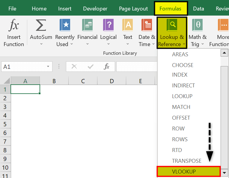
First, choose an empty cell → select the “Formulas” tab → go to the “Function Library” group → click the “Lookup & Reference” option drop-down → select the “VLOOKUP” function, as shown below.

Advanced Excel Formulas - FAQ 1

2. Where is the INDEX function found in Excel?

The INDEX function is found as follows:

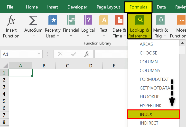
First, choose an empty cell → select the “Formulas” tab → go to the “Function Library” group → click the “Lookup & Reference” option drop-down → select the “INDEX” function, as shown below.

Advanced Excel Formulas - FAQ 2

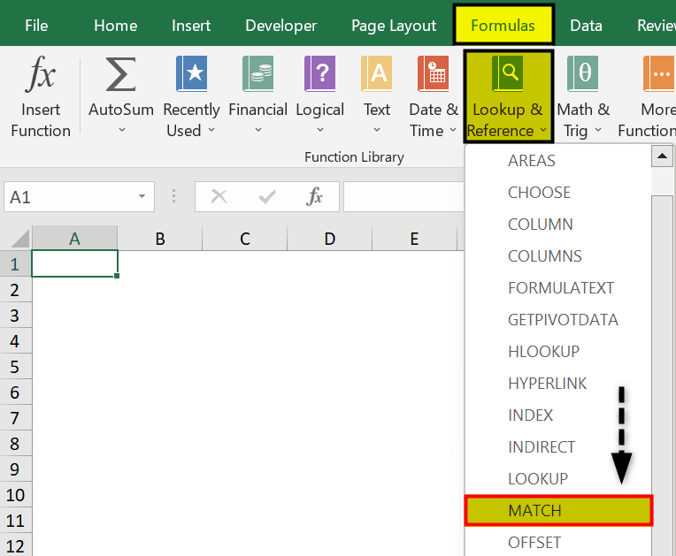
3. Where is the MATCH function found in Excel?

The MATCH function is found as follows:

First, choose an empty cell → select the “Formulas” tab → go to the “Function Library” group → click the “Lookup & Reference” option drop-down → select the “MATCH” function, as shown below.

Advanced Excel Formulas - FAQ 3

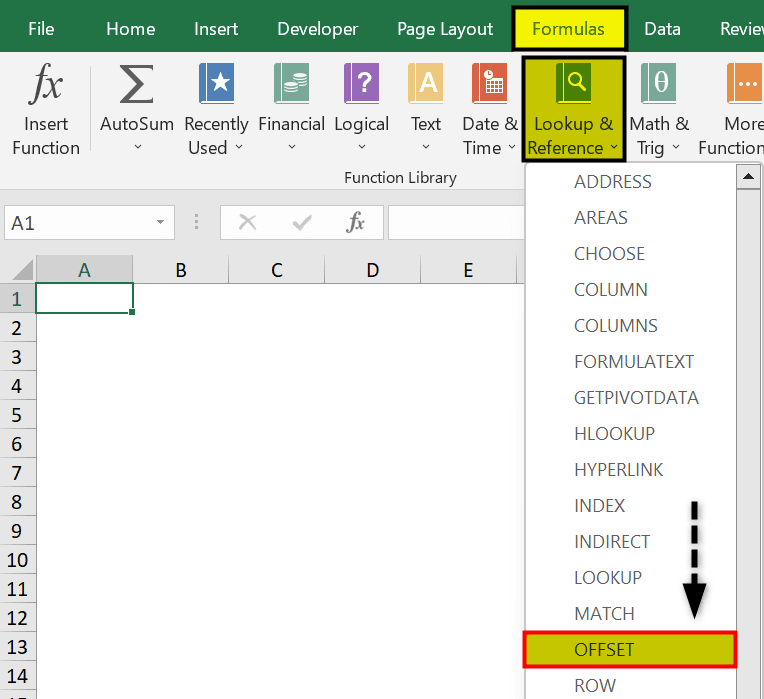
4. Where is the OFFSET function found in Excel?

The OFFSET function is found as follows:

First, choose an empty cell → select the “Formulas” tab → go to the “Function Library” group → click the “Lookup & Reference” option drop-down → select the “OFFSET” function, as shown below.

Advanced Excel Formulas - FAQ 4