What is Multiply Formula in Excel?

Last Updated :

21 Aug, 2024

Blog Author :

Edited by :

Reviewed by :

Table Of Contents

There is no in-built multiplication formula in Excel. Multiplication in excel is performed by entering the comparison operator “equal to” (=), followed by the first number, the “asterisk” (*), and the second number. In this way, it is possible to carry out the multiplication operation for a cell, row or column. For example, the formula “=16*3*2” multiplies the numbers 16, 3, and 2. It returns 96.

The arithmetic operator “asterisk” (*) is known as the multiplication symbol. It is placed between the numbers to be multiplied.

In multiplication, the number to be multiplied is known as the multiplicand. The number by which the multiplicand is multiplied is known as the multiplier. The multiplier and the multiplicand are also called factors. Their output of multiplication is known as the product.

In Excel, multiplication can be performed in the following ways:

With the "asterisk" symbol (*)
With the PRODUCT function
With the SUMPRODUCT function

Note: The SUMPRODUCT function multiplies and then sums the resulting products.

How to Use Multiply Formula in Excel?
Frequently Asked Questions
Recommended Articles

How to Use Multiply Formula in Excel?

Example #1 – Multiply Excel Columns With the “Asterisk”

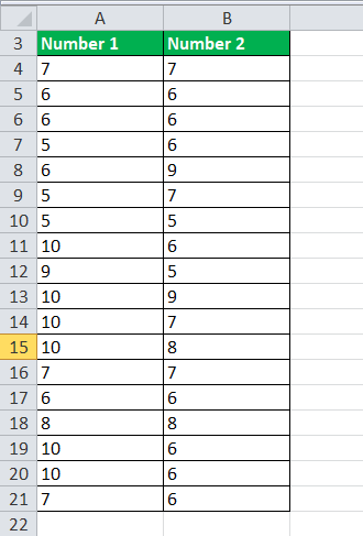
The following table shows two columns titled “number 1” and “number 2.” We want to multiply the numerical values of the first column by the second one.

Step 1: Enter the multiplication formula in excel “=A4*B4” in cell C4.

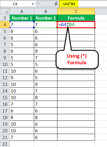
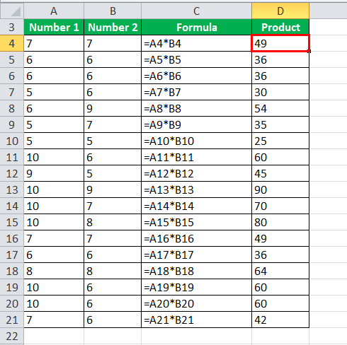
Step 2: Press the “Enter” key. The output is 49, as shown in the succeeding image. Drag or copy-paste the formula to the remaining cells.

For simplicity, we have retained the formulas in column C and given the products in column D.

Example #2 – Multiply Excel Rows With the “Asterisk”

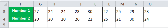
The following table shows two rows titled “number 1” and “number 2.” We want to multiply the numerical values of the first row by the second one.

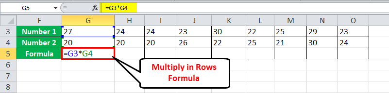
Step 1: Enter the multiplication formula “=G3*G4” in cell G5.

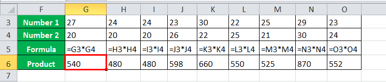
Step 2: Press the “Enter” key. The output is 540, as shown in the succeeding image. Drag or copy-paste the formula to the remaining cells.

For simplicity, we have retained the formulas in row 5 and given the products in row 6.

Example #3 – Multiply With the PRODUCT Function

The PRODUCT function can be given a list of numbers as arguments to be multiplied.

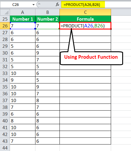
Working on the data of example #1, we want to multiply the numerical values of the two columns with the help of the PRODUCT function.

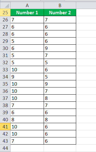
Step 1: Enter the formula “=PRODUCT (A26,B26)” in cell C26.

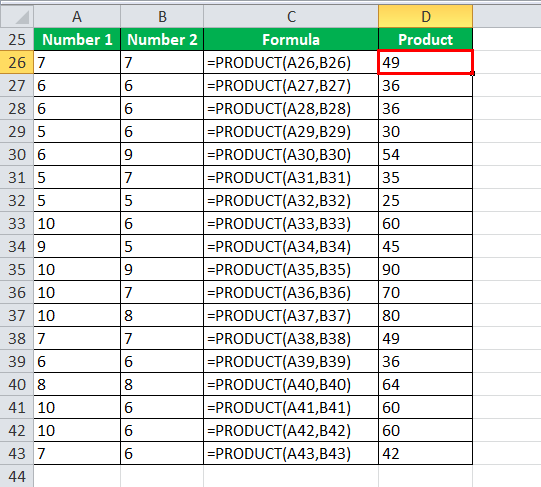
Step 2: Press the “Enter” key. The output is 49, as shown in the succeeding image. Drag or copy-paste the formula to the remaining cells.

For simplicity, we have retained the formulas in column C and given the products in column D.

Example #4 – Multiply and Sum With the SUMPRODUCT Function

With the SUMPRODUCT function, the numbers of two columns or rows are multiplied and the resulting products are summed up.

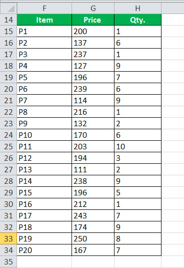
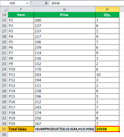
The following table shows the prices (in $ per unit) and quantities sold of 20 items. We want to calculate the total sales revenue generated by the organization.

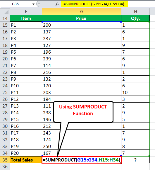
Step 1: Enter the formula “=SUMPRODUCT (G15:G34,H15:H34).”

To calculate the sales revenue, the prices are multiplied by the quantity sold. Thereafter, the resulting products are added by the given formula.

Step 2: Press the “Enter” key. The output is $20,338.

For simplicity, we have retained the formula in cell G35 and given the result in cell H35.

Example #5 – Multiply With Percentages

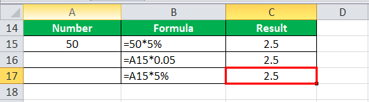
The following table shows a number in column A. We want to multiply this by 5%.

Step 1: Enter any of the following three formulas:

“=50*5%”
“=A15*0.05”
“=A15*5%”

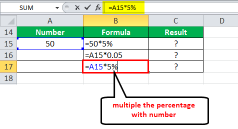
Step 2: Press the “Enter” key. The output is 2.5 with all the three formulas. It is shown in the following image.

For simplicity, we have retained the formulas in column B and given the results in column C.

Frequently Asked Questions

1. What is the multiplication formula and how to multiply in Excel?

There is no universal formula for multiplication in Excel. However, Excel facilitates multiplication with the use of the “asterisk” (*) and the PRODUCT function.

The formula using the “asterisk” is stated as follows:
“=number 1*number 2”

This is the simplest approach to multiplication that helps multiply numbers, cell references, rows, and columns.

The syntax using the PRODUCT function is stated as follows:

“=PRODUCT(number1,, …)”

The “number1” and “number2” arguments can be in the form of numbers, cell references or ranges. Only the “number1” argument is required.

The steps to multiply in Excel are listed as follows:

• Enter the comparison operator “equal to” (=).
• Enter the multiplication formula.
• Press the “Enter” key to obtain the output.

Note: A maximum of 255 arguments can be provided to the PRODUCT function.

2. How to multiply in Excel without using the formula?

Let us multiply the numbers 4, 15, 23, and 54 (in the range A2:A5) by the constant 2 (in cell B2) without using the formula.

The steps to multiply in excel with “paste special” are listed as follows:
• Select cell B2 and press the keys “Ctrl+C” to copy it.
• Select the range A2:A5, which is to be multiplied.
• Right-click the selected range and choose “paste special.”
• In the “paste special” window, select “multiply” under “operation.”
• Click “Ok.”
The outputs 8, 30, 46, and 108 are obtained in the range A2:A5.

Note: If you do not want the range A2:A5 to be overridden with new values, copy-paste the numbers of this range to a separate column. This is to be done at the beginning of the mentioned procedure.

3. How to multiply two columns in Excel?

Let us multiply column A consisting of 5, 18, 26, and 44 (in the range A2:A5) by column B consisting of 6, 4, 9, and 2 (in the range B2:B5).

The steps to multiply two columns in excel using the multiplication symbol or the PRODUCT formula are listed as follows:

• Enter the formula “=A2*B2” or “=PRODUCT(A2,B2)” in cell C2.
• Press the “Enter” key. The output 30 appears in cell C2.
• Drag or copy-paste the formula to the remaining cells.

The outputs 30, 72, 234, and 88 are obtained in the range C2:C5.

Note: Since relative references are being used, the cell reference changes as the formula is copied.

The steps to multiply two excel columns using the array formula are listed as follows:

• Select the entire range C2:C5 where you want the output.
• Enter the formula “=A2:A5*B2:B5” in the selected range.
• Press the keys “Ctrl+Shift+Enter” together. The curly braces {} appear in the formula bar.

The outputs 30, 72, 234, and 88 are obtained in the range C2:C5.