Table Of Contents
The Subtraction Formula of Excel
The subtraction formula in excel facilitates the subtraction of numbers, cells, percentages, dates, matrices, times, and so on. It begins with the comparison operator “equal to” (=) followed by the first number, the minus sign, and the second number. For example, to subtract 2 and 5 from 15, apply the formula “=15-2-5.” It returns 8.
In subtraction, the first number is the minuend (from which a number has to be subtracted) and the second number is the subtrahend (the number to be subtracted). The resulting number is the difference.
The arithmetic operator “minus” (-) is placed between the minuend and the subtrahend.
How to Use the Subtraction Formula in Excel?
The subtraction formula of Excel is easy to use. Let us go through the following examples to understand its working.
Example #1
The following table shows some values in columns A and B. We want to subtract the values in column B from those of column A.
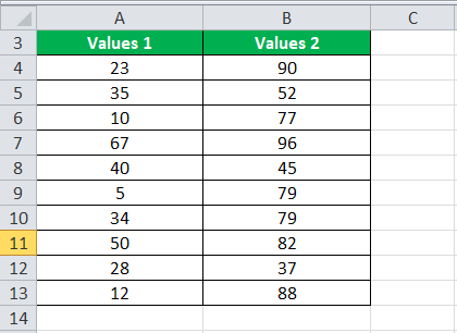
The steps to subtract the values of column B from those of column A are listed as follows:
- Enter the comparison operator "equal to" (=), followed by the cell B4, the "minus" sign (-), and the cell A4. Press the "Enter" key. The output is 67.
Note: The references B4 and A4 can either be typed or selected by clicking on the respective cells.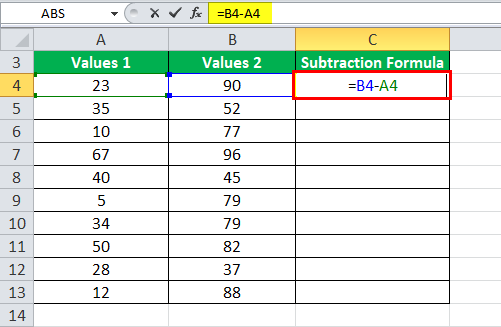
- Apply the subtraction excel formula to the remaining values. Alternatively, drag the formula of C4 till C13, as shown in the following image.
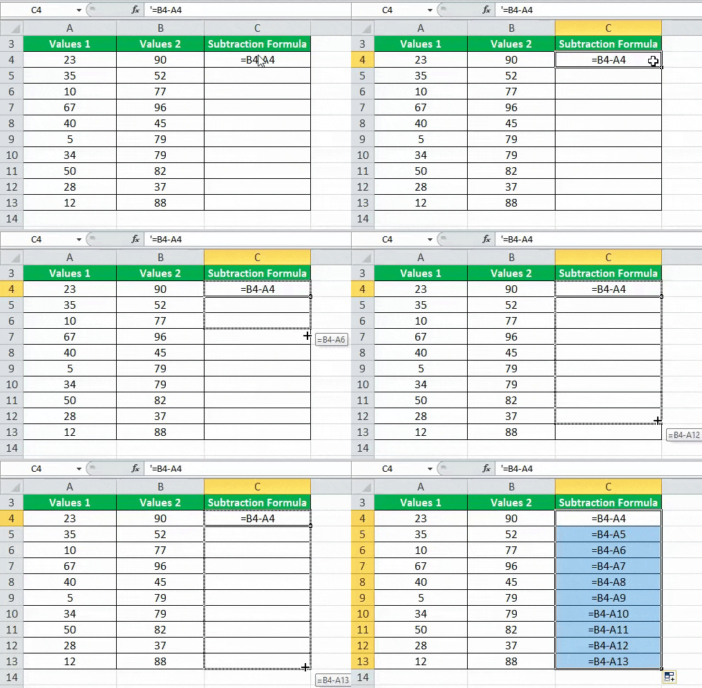
- The final output appears, as shown in the following image. For simplicity, we have retained the formulas in column C and given the differences in column D.
Note: If the values in column A or column B change, the result is automatically updated in column D.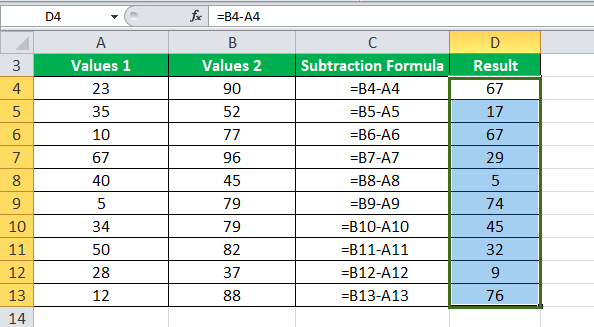
Example #2
The following table shows the names and the revenues generated (in Rs.) by ten employees of an organization. It has been decided to award Rs. 10,000 worth vouchers to those employees who have achieved the sales target of Rs. 5000.
Find the employees eligible for the reward.
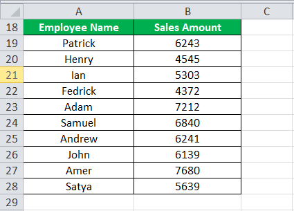
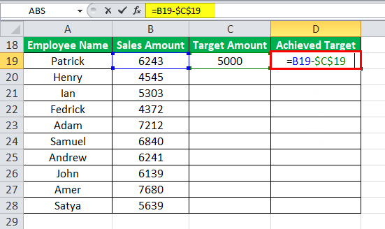
Step 1: Enter the following formula.
“=B19-$C$19”
To calculate the revenue generated over and above the target (Rs. 5000), we subtract the latter (column C) from the former (column B). Since the target amount is the same for all the employees, we use the absolute reference $C$19.
Note: In absolute cell reference, the dollar sign ($) is placed before the column letter and the row number like in $C$19. This keeps the column and the row constant.
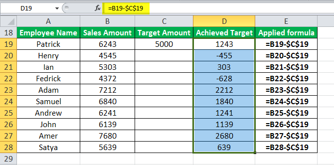
Step 2: Press the “Enter” key. The final output appears in column D, as shown in the following image.
For simplicity, we have retained the formulas in column E and given the differences in column D. The employees who have negative difference values (column D) are not eligible for the reward.
Hence, Henry and Fedrick are not eligible while the rest of them receive the gift voucher.
The Rules Governing the Subtraction Excel Formula
- It always begins with the comparison operator “equal to” (=).
- It requires the insertion of the arithmetic operator “minus” (-) between two values.
- It is used in both, simple and advanced mathematical problems where a comparison between two values is required.
- It can be used in combination with other arithmetic operators like “plus” (+), “percent” (%), “forward slash” (/), “asterisk” (*), and so on.

