Excel PERCENTRANK Function

Last Updated :

21 Aug, 2024

Blog Author :

Edited by :

Reviewed by :

Table Of Contents

PERCENTRANK Function in Excel

The PERCENTRANK function gives the rank to each number against overall numbers in percentage numbers. Not many of us use this Excel PERCENTRANK function because of a lack of knowledge, or maybe the situation never demanded this at all. But this will be a great function because showing the rank in percentage values within the data set will be a new trend.

For example, suppose we have a dataset that shows the scores of the students. And now, we need to calculate the percentile rank of each student's score. Using the Excel PERCENTRANK function, we can calculate the rank of each student's score in the dataset as a percentage of the whole dataset.

PERCENTRANK Function in Excel

Syntax

Below is the syntax of the PERCENTRANK function.

Array: This is the range of value against which we are giving rank.

x: This is nothing but the individual value from the lot.
: It is an optional parameter. We can use this argument if we want to see decimal places. For example, if the rank percentage is 58.56% and we want to see two-digit decimal values, we can enter the significance number as 2. It will show the percentage as 58.00%. It will take three digits of significance by default if you ignore it.

Examples

Example #1

Let us start the example with a simple series of numbers. Consider the below series of numbers for this example.

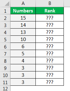
Copy and paste the above data to a worksheet.

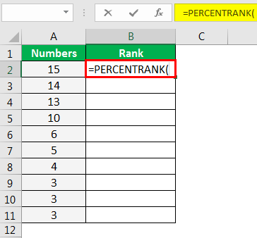
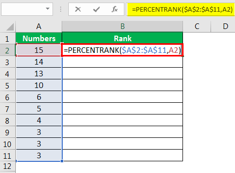
Open PERCENTRANK function

We must first open the Excel PERCENTRANK function in cell B2.
Select Number of Range as Absolute Reference

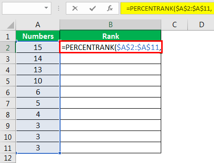
The first argument of the PERCENTRANK function is “Array,” i.e., our total numbers range from A2 to A11, so select this range as the reference and make it an absolute reference.
Now, select x reference value.

Next, we must select cell A2 as the x reference. As of now, ignore argument, and close the bracket.
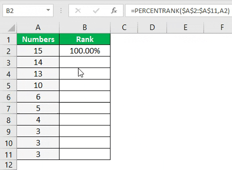
Next, press the Enter key to get the result.

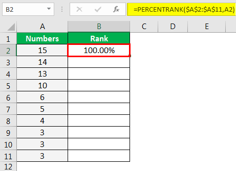
Also, drag the formula to the below cells as well.

Now, closely look at the numbers. Let us go from the bottom.

We have number 3 for the first three values, so the first lowest number in the array always ranks as 0.000%.

PERCENTRANK Function in Excel Example 1.5

Let us now go to the next value, 4. This number is ranked as 33.333% because number 4 is the 4th positioned number in the range of values. Below this number 4, there are 3 values. And above this number, there are 6 values, so the percentage is arrived at using the below equation.

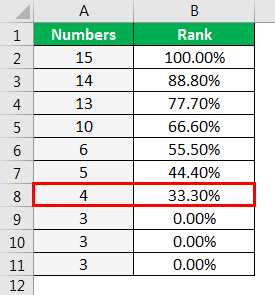
PERCENTRANK Function in Excel Example 1.6

Percentage Rank = Number of Values below / (Number of Values below + Number of Values Above)

i.e. 3 / (3 + 6)

= 33.333%

Similarly, the top value in the range is 15, and it is ranked as 100%, which is equivalent to a rank of 1.

Example #2

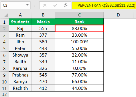
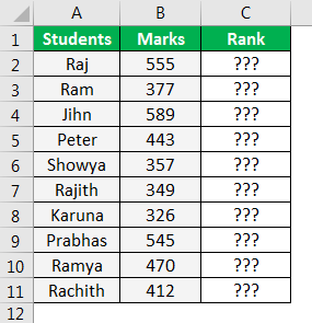
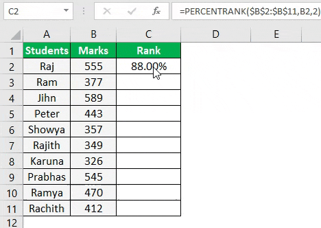
Now, look at the below scores of students in an examination.

Using this data, we will find the percentage rank. Below is the formula applied for these numbers.

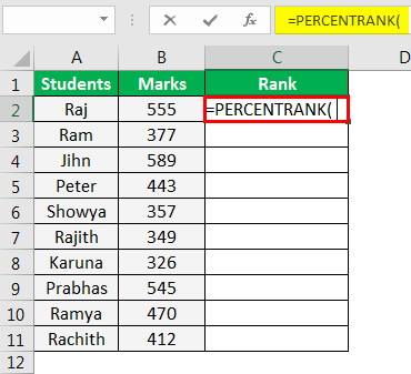
Step 1: Open the PERCENTRANK function

We must first open the PERCENTRANK function in cell C2.

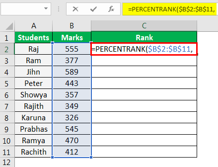
Step 2: Select Number of Range as Absolute Reference

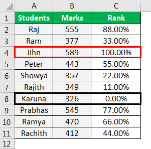
The first argument of the PERCENTRANK function is "Array," i.e., our total numbers range from B2 to B11. So, we must select this range as the reference and make it an absolute reference.

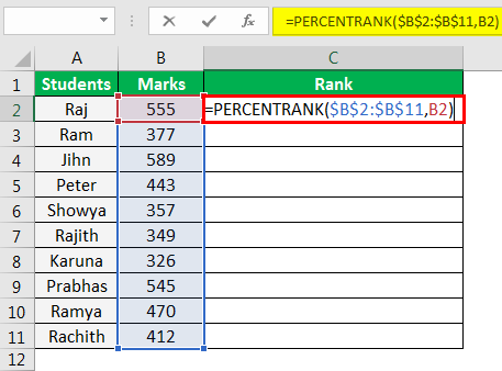
Step 3: Now select x reference value.

Next, we must select cell B2 as the "x" reference. As of now, ignore argument, and close the bracket.

PERCENTRANK Function in Excel Example 2.3

Step 4: Hit the Enter key to get the result.

Also, drag the formula to the below cells.

The lowest value in the range is 326 (B8 cell). It has a rank of 0.00%, and the highest value in the range is 589 (B4 cell). Therefore, it has been given a rank of 100%.

PERCENTRANK Function in Excel Example 2.6

We will give the significance parameter as 2 and see what happens.

The decimal places are rounded to the below number, as we can see above. So, for example, in cell C2, without using a parameter, we have got 88.80%, but this time we have got only 88.00% because of the significant value of 2.

Things to Remember Here

We must remember that only numerical values work for this function.
If the significance value is <=0, we will get #NUM! Error.
The Array and the "x" value should not be empty.