What Is Excel Statistics?
In the modern data-driven business world, we have sophisticated software dedicatedly to working towards “Statistical Analysis.” Amidst all these modern, technologically advanced excel software is not a bad tool to do your statistical analysis of the data. Of course, we can do all statistical analysis using Excel, but you should be an advanced Excel user. This article will show you some basic to intermediate-level statistics calculations using Excel.
How To Use Excel Statistical Functions?
#1: Find Average Sales Per Month
The average rate or trend is what the decision-makers look at when they want to make crucial and quick decisions. So finding the average sales, cost, and profit per month is a common task everybody does.
For example, look at the below data of monthly sales value, cost value, and profit value columns in Excel.
So, by finding the average per month from the whole year, we can see what per month numbers are.
Using the AVERAGE function, we can find the average values from 12 months, which boils down to per month on an average.
- Open the AVERAGE function in the B14 cell.
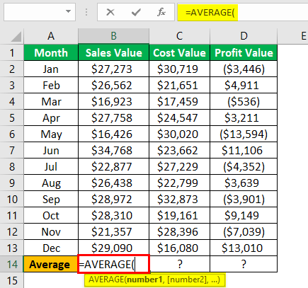
- Select the values from B2 to B13.
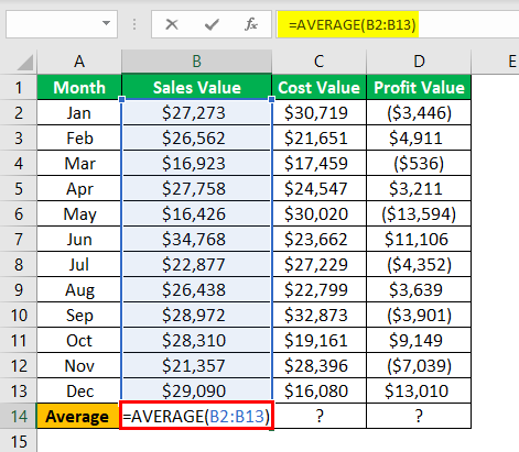
- The average value for sales is:
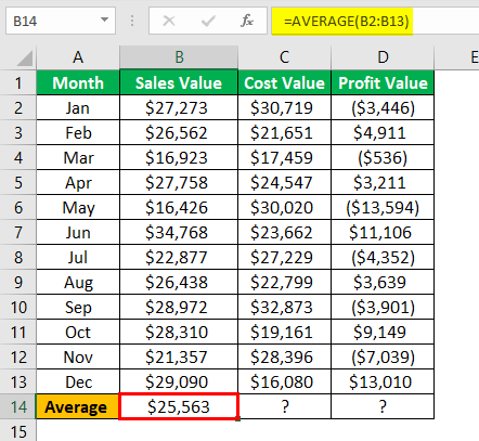
- Copy and paste cell B14 to the other two cells to get the average cost and profit. The average value for the cost is:

- The average value for the profit is:
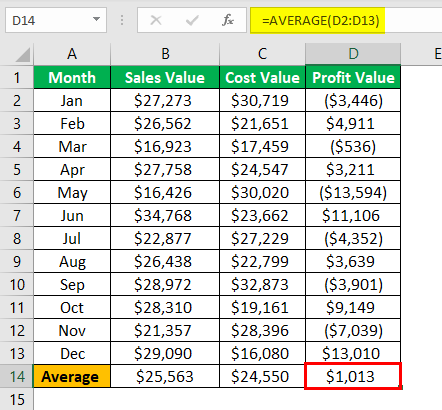
So, on average, per month, the sale value is $25,563, the cost value is $24,550, and the profit value is $1,013.
#2: Find Cumulative Total
Finding the cumulative total is another set of calculations in excel statistics. Cumulative is nothing but adding all the previous month’s numbers together to find the current total for the period.
The steps to find the cumulative total are as follows:
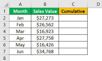
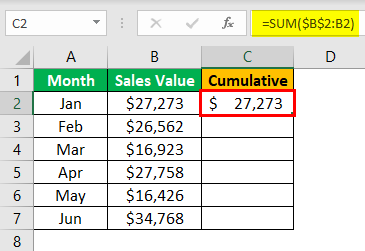
- First, look at the below 6 months sales numbers.

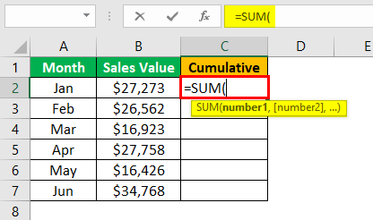
- Open the SUM function in the C2 cell.

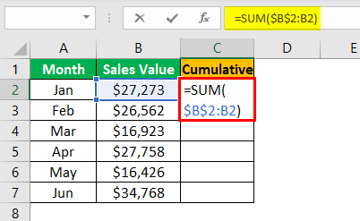
- Select the cell B2 cell and make the range reference.
From the range of cells, make the first part of the cell reference B2 an absolute reference by pressing the F4 key.

- Close the bracket and press the “Enter” key.

- Drag and drop the formula below one cell.

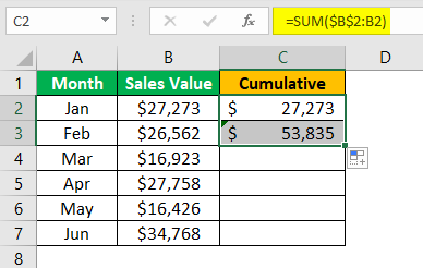
- Now, we have the first two months’ cumulative total. At the end of the first two months, revenue was $53,835. Drag and drop the formula to other remaining cells.
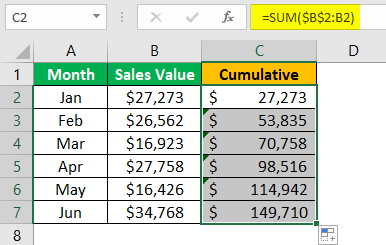
From this cumulative, we can find in which month there was a less revenue increase.

#3: Find Percentage Share
Out of twelve months, you may have got $1,000,000 in revenue. But, still, maybe in one month, you must have achieved the majority of the revenue, and finding the month’s percentage share helps us find the particular month’s percentage share.
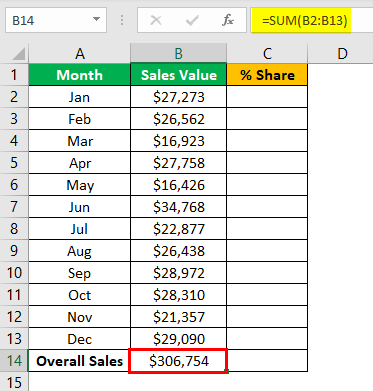
For example, look at the below data of the monthly revenue.
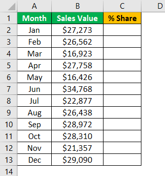
To find the percentage share first, we need to see what the overall 12 months total is, so by applying the SUM function in Excel, find the overall sales value.
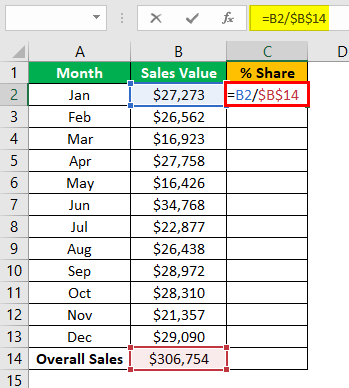
We can use the formula to find the percentage share of each month.
% Share = Current Month Revenue / Overall Revenue
To apply the formula as B2 / B14.
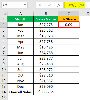
The percentage share for Jan month is:
Note: Make the overall sales total cell (B14 cell) an absolute reference because this cell will be a common divisor value across 12 months.
Copy and paste the C2 cell to the below cells as well.
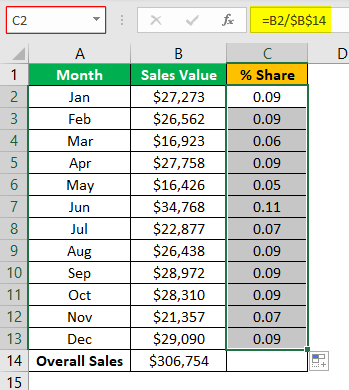
Apply the “Percentage” format to convert the value to percentage values.
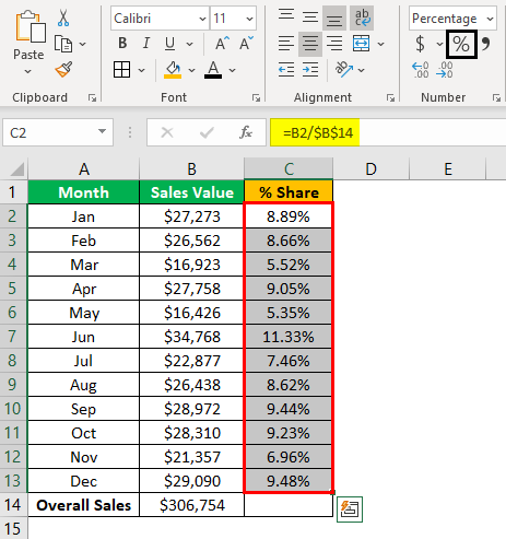
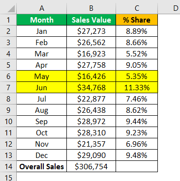
So, from the above percentage share, we can identify that the “Jun” month has the highest contribution to overall sales value, i.e., 11.33%, and the “May” month has the lowest contribution to overall sales value, i.e., 5.35%.
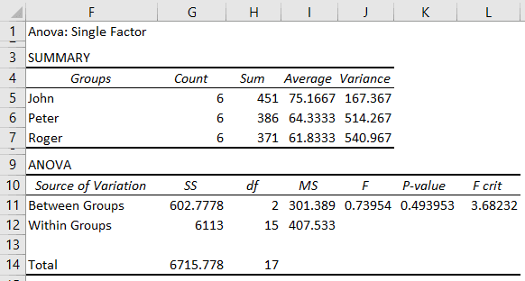
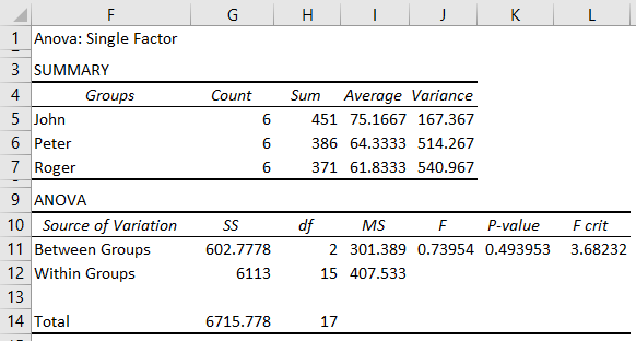
#4: ANOVA Test
Analysis of Variance (ANOVA) is the statistical tool in excel used to find the best available alternative from the lot. For example, if you are introducing four new kinds of food to the market. You gave a sample of each food to get the public’s opinion and from the opinion score given by the public by running the ANOVA test. We can choose the best from the lot.
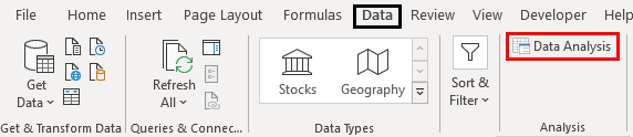
ANOVA is a data analysis tool available in Excel under the “DATA” tab. By default, it is not available. You need to enable it.
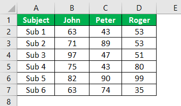
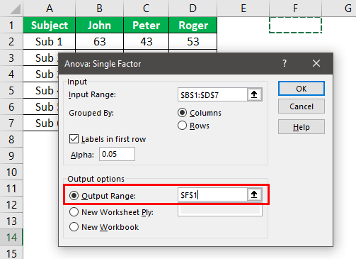
Below are the scores of three students from 6 different subjects.
Click on the “Data Analysis” option under the “Data” tab. It will open up below the “Data Analysis” tab.
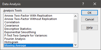
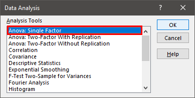
Scroll up and choose “Anova: Single Factor.”
Choose “Input Range” as B1 to D7 and tick “Labels in first row.”
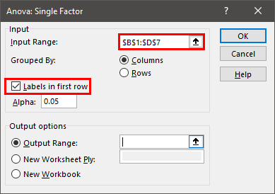
Select the “Output Range” as any of the cells in the same worksheet.
We will have an “ANOVA” analysis ready.
Important Things To Note
- All the basic and intermediate statistical analyses are possible in Excel.
- We have formulas under the category of “Statistical” formulas.
- If you are from a statistics background, it is easy to do fancy and important statistical analyses in Excel like T-TEST, Z-TEST, descriptive statistics, etc.
Key Takeaways
- Statistics in Excel refers to conducting statistics analysis using Microsoft Excel.
- Excel provides all the fundamental and analytical statistical analysis with formulas under the category “Statistical” formulas.
- Excel also enables easy and accessible advanced statistical analyses such as T-TEST, Z-TEST, and Descriptive Statistics. It can be beneficial for professionals who are from statistical backgrounds.
Frequently Asked Questions (FAQs)
How to get regression statistics in Excel?
To get the regression statistics in Excel for your data, you need to navigate to the “Data” menu and then select the “Data Analysis” tab. Consequently, you will find a listing of different statistical tests that Excel has to offer. Then, after that, scroll down to search the regression option and hit the “OK” button. Then, finally, insert the cells that possess data in Excel.
How do you track statistics in Excel?
To track the statistics in Microsoft Excel, choose the “Review” tab, and in the “Proofing section,” choose “Workbook Statistics.” You can also opt for the shortcut “CTRL+SHIFT+G” to complete the task, but remember that this shortcut would not work in Excel for the web. On pressing this shortcut, the “Workbook Statistics” dialog box will appear and show counts and various other details concerning the current worksheet and current workbook.
How to graph statistics in Excel?
To graph statistics in Excel, you must first click on the Excel data that you need to plot and then select the data and choose Insert>Charts>, and then finally choose the chart type of your choice from the available menu that displays to you.
Recommended Articles
This article is a guide to statistics in excel. Here, we discuss using Excel statistical functions, practical examples, and a downloadable Excel template. You may learn more about Excel from the following articles: –