Time Value of Money

Last Updated :

Blog Author :

Edited by :

Reviewed by :

Table Of Contents

Time Value of Money Definition

Time Value of Money (TVM) is a fundamental financial concept, stating that the current value of money is higher than its future value, given its potential to earn in the years to come. Thus, it suggests that a sum of money in hand is greater in value than the same sum of money received in the next couple of years.

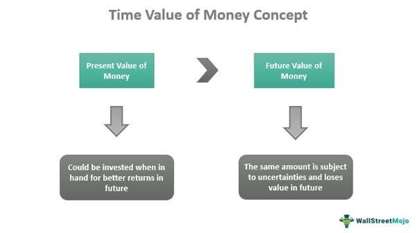
Also referred to as the present discounted value, TVM is determined by its ability to yield returns in terms of its future value. A person having the money in hand can invest it for better returns in the future. On the other hand, the same amount received a year after, it loses its value.

Time Value of Money Definition

Time Value of Money (TVM) is the basic financial concept that advocates how the current value of money is higher than its value in the future.
It is the potential earning capacity of the money that decides its current and future value.
TVM helps investors make the best investment decisions, knowing the future returns they should expect from what they invest.
Money loses its value over time, which causes inflation affecting the buying power of the public.

Time Value of Money Explained

Time Value of Money comprises one of the most significant concepts in finance. The idea focuses on identifying the real value of cash flows expected in the future due to the business or individual investment decisions made from time to time.

For example, A wins a lottery of $1,000 and has two options to either take a lump sum right at the moment or receive the same after a year or two. It is obvious for the winner to choose the first option as the winner can invest that money and receive $1,200 or more in the next two years. But, on the other hand, if A chooses to go otherwise, it will be the same $1,000 even after two years.

TVM is an important factor in determining the purchasing power, and hence it is considered an important concept in inflation. TVM is hugely affected during inflation as the latter hampers the purchasing power of money, leading to the loss of its value.

Time Value of Money Explained in Video

Formula

The Time Value of Money formula is expressed below:

Or,

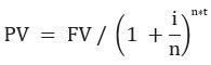
Here,

PV = Present value of money
FV = Future value of money
i = Rate of interest or current yield on similar investment
t = No. of years
n = No. of compounding periods of interest each year

Example

Let us understand the TVM calculation through the following Time Value of Money example:

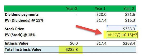
Mario purchases a stock expected to pay dividends of $20 (Div 1) next year and $21.6 (Div 2) the following year. As he receives the second dividend, he plans to sell the stock for $333.3. What is the intrinsic value of this stock if the required return is 15%?

To make sure the required return is 15%, Mario attempts to find out the stock's intrinsic value.

First, the investor calculates the present value of Dividends for Year 1 and Year 2.

Using the above formula, he gets,

Present Value (Year 1) = $20/ ((1.15) ^ 1)
Present Value (Year 2) = $20 / ((1.15) ^2)
In this example, they come out to be $17.4 and $16.3, respectively, for 1st and 2nd-year dividends.

Secondly, he computes the present value of future selling price after two years.

PV (Selling Price) = $333.3 / (1.15^2)

= 252.0

Now, Mario adds the present value of dividends and the present value of selling price to get the intrinsic value of the stocks

Present Value (Year 1) + Present Value (Year 2) + Present Value (Selling Price)

= $17.4 + $16.3 + $252.0

= $285.8

Time Value of Money Analysis

The Time Value of Money concept determines the potential earning capacity of an amount in the future. It, therefore, helps different financial sectors to understand and compute the present value and compare the same with the future value of a particular amount. Based on the results obtained, they decide whether to invest in a particular venture, asset, or security.

The financial firms use this idea of TVM for the following purposes:

It helps in comparing the investment alternatives available in the market. Investors assess the returns and other conditions to make a final decision on what option to choose.
Investors choose the best investment proposals based on the evaluation, considering the TVM.
Lenders decide the interest rates for loans, mortgages, etc., based on the present and future value of an amount.
The value of money, when known, helps in fixing appropriate wages and prices of products.

In addition, the changing value of an amount also plays a considerable role in determining when a particular investment matures or when to repay a loan amount, etc.

Frequently Asked Questions (FAQs)

What is the Time Value of Money?

TVM is the fundamental financial concept that revolves around the changing value of money over time. It states how the present value of money is greater than its future value. The value that money holds currently and in the future is assessed based on its potential earning capacity.

Why is TVM important?

The three main reasons that make TVM an important concept are – inflation, risk or uncertainty, and liquidity.

• Inflation is the loss of purchasing power caused by the deteriorating future value of money.
• Risk or uncertainty is the difference between what is received as an outcome and expected when the investment or expenditure was made.
• Liquidity makes it easy for owners to sell their assets for cash as illiquid assets are difficult to sell.

How does TVM affect financial decision-making?

Calculating TVM is important as it helps financial sectors make suitable investment decisions. Using the concept, the key investors compare the available investment options and choose the best alternatives to invest in. Then, given the expected loss in the value of money, the rate of interest and tenure of repayment for loan and mortgage schemes are determined. In addition, determining TVM also helps fix the wages of workers and prices of consumer goods.