What Are HLOOKUP Examples In Excel?
HLOOKUP Examples in Excel are the examples of the datasets retrieved using the Horizontal Lookup or the HLOOKUP function in Excel. However, before we consider examples of the HLOOKUP function, we must first understand the formula and the function.
HLOOKUP Examples Excel Template
Download Excel TemplateFor example, in a dataset, to get the salary of the Emp ID – ID148 we apply the HLOOKUP function in cell A8.

We get the output, as shown above.
The Formula Of HLOOKUP FUNCTION In Excel
The syntax of the HLOOKUP formula is,
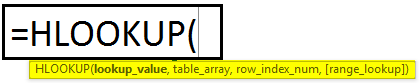
The arguments of the HLOOKUP formula are,
- lookup_value: We consider this a base value to find the required result.
- table_array: This data table has a lookup value and a result value.
- row_index_num: It is where our result is in the data table.
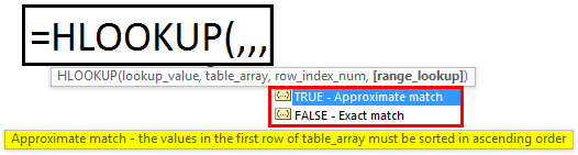
- [range_lookup]: Here, we have two parameters. The first one is TRUE (1), which finds an approximate match from the table, and the second one is FALSE (0), which sees the exact match from the table.
- The TRUE parameter can be passed as number 1.
- The FALSE parameter can be passed as number 0.
- The HLOOKUP examples helps us understand one of the important LOOKUP functions i.e., the horizontal or HLOOKUP formula.
- Data table structure matters a lot. If the data table is horizontal, then HLOOKUP should be applied. If the table is vertical, then we should use the VLOOKUP function.
- We also have another function, the XLOOKUP, which combines the HLOOKUP and the VLOOKUP functions.
- The MATCH function returns the row number of supplied values.
- INDEX + MATCH can be used as an alternative to the HLOOKUP function in Excel.
Download Template
This article must help understand HLOOKUP Examples with its formulas and examples. You can download the template here to use it instantly.
You can download this HLOOKUP Example Excel Template here – HLOOKUP Examples Excel Template
HLOOKUP Function Video Explanation

HLOOKUP Examples In Excel
Here are some examples of the HLOOKUP function in Excel.
Example #1
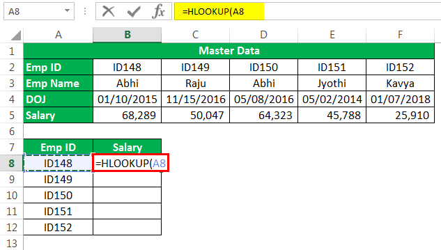
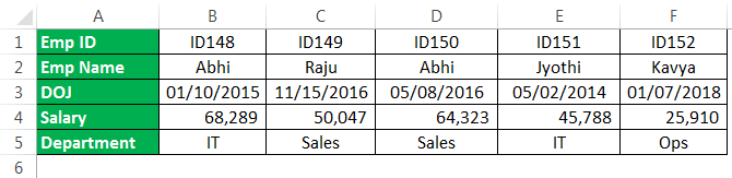
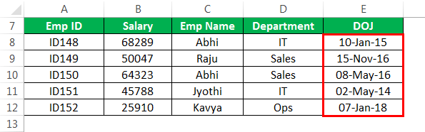
In an HR department we may deal with employees’ information like salary, DOJ, etc. as given in the data below.
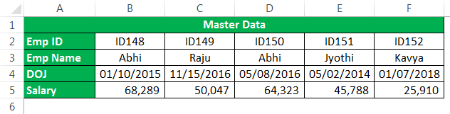
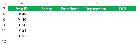
It is the master data we have. We have received the “Emp ID” from the finance team, and they have requested their salary information to process the salary for the current month.
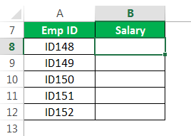
Here the main the data is in horizontal form, and the request came in vertical format.
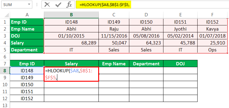
Therefore, the steps to apply the HLOOKUP function to fetch the data are,
First, we must open the HLOOKUP formula in the salary column and select the lookup value as “Emp ID.”

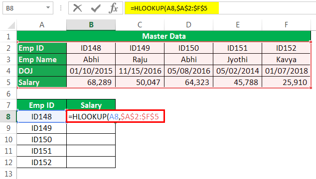
The next thing is we need to select the table array, i.e., the main table.

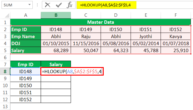
We have locked the main table range by pressing the F4 key. It has become an absolute reference now.We need to mention the row number, from which row of the main table we are looking for the data. In this example, the row number of the required column is 4.

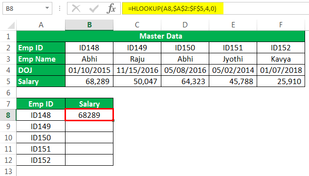
The final part is a range lookup. Since we are looking at the exact match, we need to select the option as “FALSE” or “zero” (0).

We are done. We got the value we required through the HLOOKUP function.
Now, drag the formula to get the result to the rest of the cells.

Example #2 – HLOOKUP + MATCH Formula
We have added the department against each employee’s name here for the same data as above.
We have another table that requires all the information based on the Emp ID, but all the data columns are not in order.
If we manually supply row numbers, we must keep editing the formula for all the columns. Instead, we can use the MATCH formula to return the row number based on the column heading.
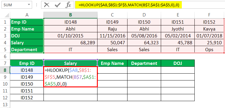
We must apply the MATCH function in the row index number and automatically get the row numbers. Then, use the formula as shown in the below image.

Mention the final argument and close the formula.
We get the following result.
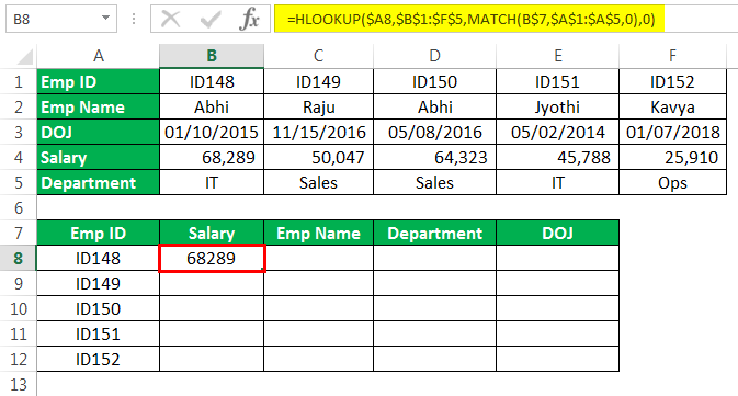
Now, drag the formula to other cells. We will have the final results.
One problem here is we do not get the format for the date column. So, we need to use the date format in excel manually.
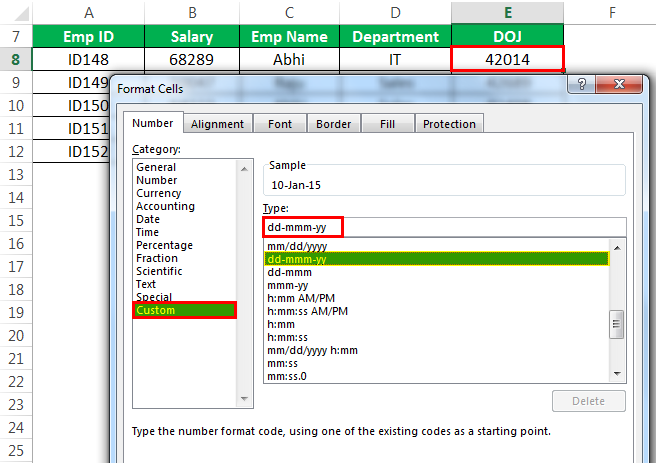
Apply the above format to the date column. We will have the correct date values.
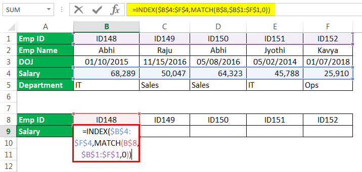
Example #3 – INDEX + MATCH as the Alternative to HLOOKUP
We can apply the MATCH + INDEX function as the alternative to get the result instead of the HLOOKUP function. Let us consider the below screenshot of the formula.
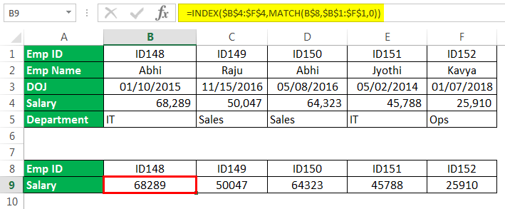
The output is given below:
Important Things To Note
- We will get an #N/A error if the lookup_value is not the exact value in the data table.
- If we do not provide the value as 0 or 1 for the last argument in the HLOOKUP formula, by default, it will take 0, and return an exact match.
- If the row index number is not in the range formula, we will get the #REF error.
Frequently Asked Questions
1. Where is the HLOOKUP function found in Excel?
The HLOOKUP function is found as follows:
First, choose an empty cell – select the “Formulas” tab – go to the “Function Library” group – click the “Lookup & Reference” option drop-down – select the “HLOOKUP” function, as shown below.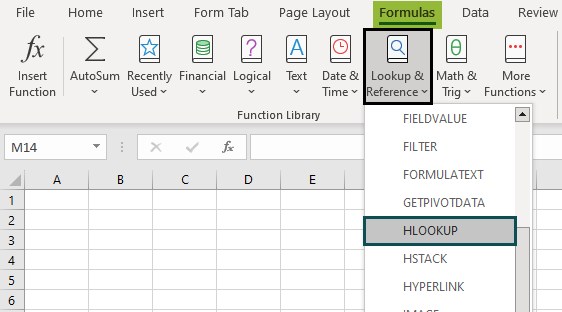
2. Where is the VLOOKUP function found in Excel?
The VLOOKUP function is found as follows:
First, choose an empty cell – select the “Formulas” tab – go to the “Function Library” group – click the “Lookup & Reference” option drop-down – select the “VLOOKUP” function, as shown below.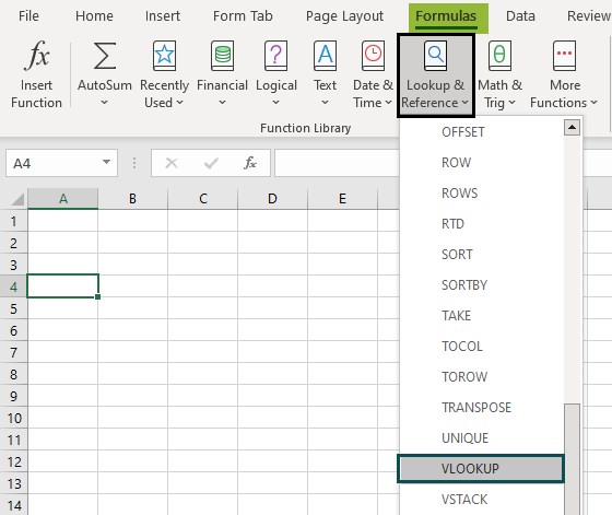
3. Where is the INDEX function found in Excel?
The INDEX function is found as follows:
First, choose an empty cell – select the “Formulas” tab – go to the “Function Library” group – click the “Lookup & Reference” option drop-down – select the “INDEX” function, as shown below.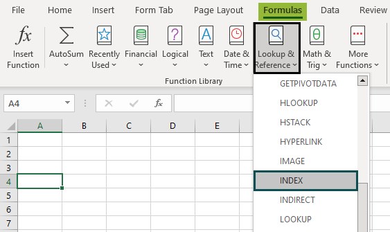
4. Where is the MATCH function found in Excel?
The MATCH function is found as follows:
First, choose an empty cell – select the “Formulas” tab – go to the “Function Library” group – click the “Lookup & Reference” option drop-down – select the “MATCH” function, as shown below.
5. Why is the HLOOKUP function not working?
A few reasons the HLOOKUP function may not work are,
• We are trying to fetch the data from bottom to top. It is not possible because, like VLOOKUP, HLOOKUP has a limitation of fetching the data from top to bottom, not from bottom to top.
• The lookup_value is not found in the table_array or dataset.
• The dataset is modified and the retrieved value where we have applied the formula, did not get updated.
• The existing dataset is deleted or removed. So, the formulas is unable to reference to give the output.
Recommended Articles
This article is a guide to HLOOKUP Examples. Here we discuss examples of HLOOKUP function, formula, and INDEX(), MATCH(), examples, downloadable excel template. You may learn more about Excel from the following articles: –