Table Of Contents
Table Array in VLOOKUP Function
In VLOOKUP or vertical lookup, when we use a reference cell or value to search in a group of columns containing data to be matched and retrieve the output, the group of the range we used to match is called VLOOKUP table_array. In the table array, the referenced cell is on the leftmost side of the column.
The VLOOKUP (vertical lookup) function in Excel looks up a piece of information or value from one column of a table array or dataset and extracts it. Then, it returns some corresponding value or information from another.
VLOOKUP in Excel is a built-in function named because the formula searches for value and searches it vertically down a specific column. It stops when it finds that value and looks to the right in a specified column.
The function needs value or arguments to run. For example, in creating an HLOOKUP or VLOOKUP function in Excel, we enter a range of cells as one of the arguments. This range is called the table_array argument.
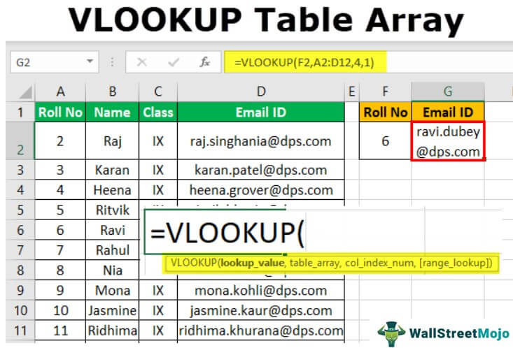
The general syntax for the VLOOKUP function is as follows:

The VLOOKUP function syntax has the following arguments:
- lookup_value: Required. It represents the value we want to look for in the first column of a table or dataset.
- table_array: Required. It represents the dataset or data array that is to be searched.
- col_index_num: Required. It represents the integer specifying the column number of the table_array that we want to return a value from
- range_lookup: Optional. It represents or defines what the function should return if it does not find an exact match to the lookup_value. This argument can be set to "FALSE" or "TRUE," where 'TRUE' indicates an approximate match (use the closest match below the lookup_value in case the exact match is not found), and "FALSE" indicates an exact match (it returns an error in case the exact match is not found). "TRUE" can also be substituted for "1" and "FALSE" for "0."
So, we can see in the above syntax that the second argument provided to the function is the VLOOKUP table_array.
Examples
Example #1
Suppose we have a student records table containing some students' roll numbers, names, class, and email IDs. Now, if we wish to get the email ID of a particular student from this database, then we use the VLOOKUP function as follows:
=VLOOKUP(F2,A2:D12,4,1)
The above formula shows the range- A2: D12 is the VLOOKUP table array.
The third argument with value 4 tells the function to return the value in the same row from the fourth column of the student records table. Finally, the last argument mentioned as 1 (TRUE) tells the function to return an approximate match (exact match if it exists).
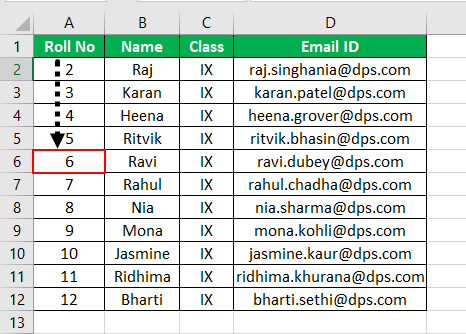
We can see that the VLOOKUP formula looks for the value 6 (as cell F2 contains the value 6) in the left-most column of the student records table by searching from top to bottom.
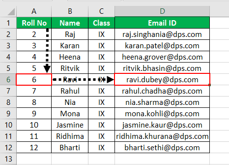
As soon as the formula finds the value 6, it goes to the right in the fourth column and extracts the email ID from it.
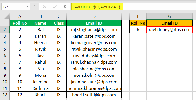
So, we can see that the email ID of roll no 6 is correctly extracted and returned with this function.
Video Explanation of VLOOKUP Excel
Explanation of VLOOKUP Excel
Example #2
Suppose we have two tables: an employee table consisting of "Employee ID," "Employee Name," "Team" of the employee, and "Designation" of the employee. Then, another table consists of some employee IDs. We wish to find their corresponding designation, so we apply the VLOOKUP formula in one cell using absolute referencing for table_array and paste it to other cells.
=VLOOKUP(F2,$A$2:$D$11,4, 1)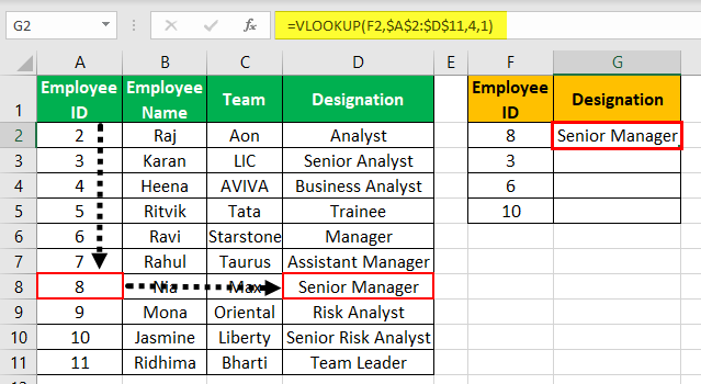
We can see that absolute referencing is created by typing a "$" in front of the row and column of a cell reference. It will allow the user to copy the cell reference to other cells while locking the reference point: (starting and ending cells of table array-A2:D11 in this case). After typing the cell reference, a keyboard excels shortcut for creating an absolute reference is by pressing the F4 key on the keypad.
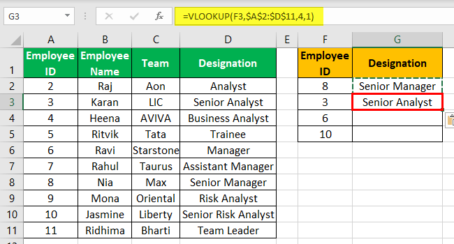
So now, when we copy the VLOOKUP formula from cell G2 and paste it down to three other cells: G3, G4, and G5. Then, only the lookup value (the first argument that has cell reference) changes, and the second argument (table_array) remains the same because, in G2, we used absolute cell referencing for table_array so that the table range remains fixed or locked.
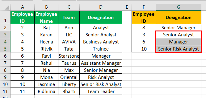
So, we can see that designation for the corresponding employees' IDs is correctly extracted and returned with absolute referencing for table_array.
Example #3
Suppose the table_array is on another worksheet (Example1) in the workbook. And the "Roll No" and corresponding "Email ID" we wish to find is on another worksheet (Example3). If this is the case, then the table_array argument in the VLOOKUP function includes the sheet name followed by an exclamation mark and cell range.
=VLOOKUP(A2,Example1!A2:D12,4, 1)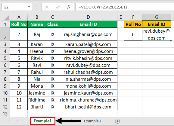
We can see that the student records table is contained in the range: A2:D12 in the worksheet named "Example1," whereas the cell and worksheet where we wish to return the value of "Roll No 12" is contained in the worksheet named "Example3." So, in this case, the second argument in the VLOOKUP function in cell B2 of worksheet "Example3" contains the sheet name with table_array followed by an exclamation mark and cell range.
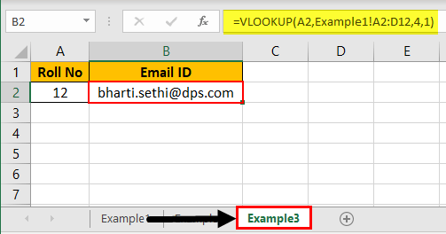
So, we can see that the email ID of roll no 12 is correctly extracted and returned even when the VLOOKUP table array is present on another workbook sheet.
Things to Remember
- The argument: table_array is always the second argument in the LOOKUP function in excel.
- The table_array argument in the LOOKUP function always follows the lookup value.
- The range of cells listed as an argument in the table_array can use absolute or relative cell references.
- Locking the VLOOKUP from a table array allows us to reference a dataset against multiple lookup values quickly.
- The cells in the table_array argument can even be present on another worksheet in the workbook. If this is the case, then the VLOOKUP table_array argument includes the sheet name followed by an exclamation mark and cell range.
- The argument "table_array" provided to the LOOKUP function must be at least as many columns wide as the value of argument "col_index_num."
- For the VLOOKUP function, the table_array must contain at least two columns of data.


