Table Of Contents
Why do we need FALSE in VLOOKUP?
In VLOOKUP, there is only one optional argument:.Using this r argument, we can provide two parameters, i.e., TRUE or FALSE.


As beginners, we may not have realized this because, at the learning stage, we are in a hurry, so this goes unnoticed.
Based on the kind of range lookup we give is important. As we have learned above, we can provide TRUE or FALSE. So, let us understand what these two arguments do.
TRUE or 1: If we provide TRUE, it will look for an approximate match.
FALSE or 0: If we provide FALSE, it will look for an exact match.
Since is an optional argument, it will take TRUE as the default parameter.
Explanation of VLOOKUP Excel Function
Now, look at the below data tables in excel.
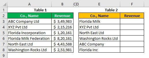
Table 1 shows the "Company Name" and its "Revenue details." However, in Table 2, we have only "Company Name," so we need to find the "Revenue" details from Table 1 based on the "Company Name" available in Table 2.
Follow the steps to use FALSE in Excel VLOOKUP.
Open the VLOOKUP function in the F3 cell.

Choose the Lookup Value as an E3 cell.

Next, choose the VLOOKUP table array as the Table 1 range.

Column Index Number as 2.

The last argument is . Mention it as TRUE or 1 in the first attempt.

For the naked eye looks like we have got revenue details for all the companies. But this is not the matching data because of the cell E3.

In this cell, we have the word “Florida Milk,” but the actual company name in Table 1 is the “Florida Milk Federation.” Even though these values differ, we still got the revenue details as $120,161. It is the revenue detail of “Florida Incorporation.”Similarly, look at the F8 cell result.

In this case, the company name is “Florida Inc,” but the actual company name is “Florida Incorporation,” so these two values are not exact. Still, because we have used the match type as TRUE, i.e., approximate match, it has returned the approximate match result.However, look at the cell F7 for the company “ABC Company.”

In this case, the lookup value is “ABC Company,” but in Table 1, we have “ABC Company Ltd” but still got the correct result. So using TRUE as the criteria for the , we cannot exactly know how it will end up. So, we need to use FALSE as the matching criteria.For the same formula, change the criteria from TRUE to FALSE (0) and see the result.

The same formula. We have only changed the criteria from TRUE to FALSE and looked at the results. We have the error values for all those cells that do not have exact lookup values, so whichever cells have the exact lookup value in Table 1 has the perfect results.
So 99.999% of the time, we need the exact matching results, so FALSE is the criteria we need to use to get exact matching results.
Video Explanation of VLOOKUP Excel Function
Things to Remember
- The need for using TRUE may not arise, so always stick to FALSE as the criteria for
- The is an optional argument. If you ignore it, it will take TRUE as the default matching criteria.
- Instead of TRUE, we can give 1 as the criteria, and instead of FALSE, we can provide 0 as the criteria.