
Table Of Contents
What Is INDEX Match Function In Excel?
The INDEX function returns a value based on a given row and column number, while the MATCH function finds the position of a specific value within a range. Together, INDEX and MATCH provide a powerful alternative to VLOOKUP, allowing for lookups in any direction, which is a limitation with VLOOKUP.
For example, to find the name of an employee with ID 100 in a list, you can use:
=INDEX(B2:B5, MATCH(100, A2:A5, 0))
Here, column A contains the employee IDs and column B contains their names.
For example, suppose we have an Excel worksheet containing the list of student's names and the corresponding scores they achieved in their exams in the range A1:B4.
If we must extract the value of cell A1 which contains the student name, “Micheal,” which is within the specified range, we can use the INDEX function.
Using the INDEX function,=INDEX(A1:B4,1,1), we can obtain the required extracted values at the intersection of the specified row and column numbers. In this scenario, on inserting the INDEX Excel function formula in cell C1, it reaches the range A1:B4 and fetches the cell's value at the intersection of the first row (row 1) and the first column (column A). The cell is A1, and its value is “Micheal.” So, the Excel INDEX function returns “Micheal.”
In the same Excel worksheet, suppose we need to know the position of the scores achieved by the student, “Micheal” Therefore, in such a scenario, we can use the Excel MATCH function. Applying the MATCH formula, “MATCH(80,A11:A15,0),” returns 1 since the score achieved by Micheal is at the first position in the Excel worksheet.
Key Takeaways
- The Index Match function allows flexible lookups by combining the ability of the MATCH function to return a value from a specific position with finding that position using INDEX in a dataset.
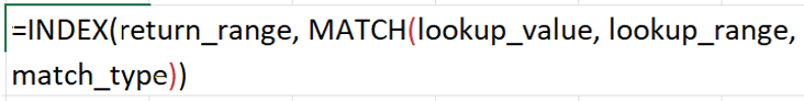
- The syntax for INDEX and MATCH combined is: =INDEX(return_range, MATCH(lookup_value, lookup_range, match_type)).
- Its advantage over VLOOKUP is that it can perform both vertical and horizontal lookups and find a match even when the lookup column is to the right.
Syntax
Since the INDEX MATCH function is not an available function by default, we have to combine the functions, INDEX and MATCH.
The syntax of the INDEX function is:
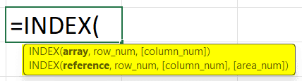
- Array: From which column or array do we need the value?
- Row Number: In the provided array, do we need the result from which row?
These two arguments are good enough in most situations.
Similarly, the syntax of the MATCH function is:
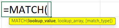
- Lookup Value: For which lookup value are we trying to find the position?
- Lookup Array: In which array or range of cells are we looking for the lookup value?
- Match Type: This will decide what kind of result we need. We can provide zero for an exact match.
The syntax for using INDEX and MATCH together is:
Index Match Function In Excel - Explained in Video
How To Use INDEX Function In Excel?
We know that the INDEX function returns the result from row number. Let us learn how this function works with the following example.
Example
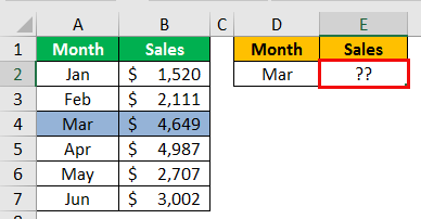
For this example, consider the below data.
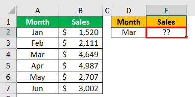
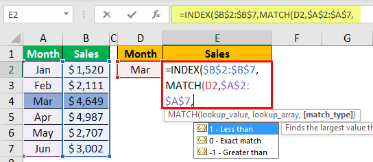
We have data from A1 to B7 cell range. In the D2 cell, we have the month name, and for this month’s name, we need sales value in cell E2.
Step 1: Let us open the INDEX function in cell E2.
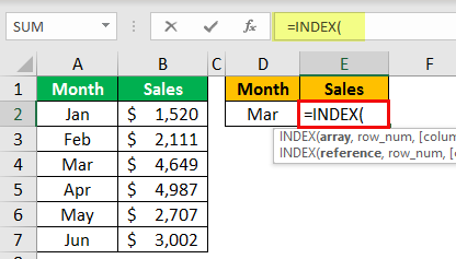
Step 2: An array is the first argument, i.e., from which column we need the result, i.e., we need results from the “sales” column, so select from B2 to B7.
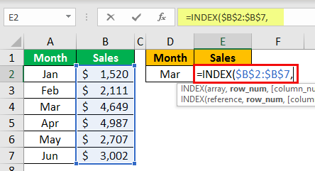
Step 3: Next is the ROW number, i.e., the selected range of cells from which row we need the result. In this example, we need the sales value for the month “Mar.” In the selected range, “Mar” is the third row, so we need results from the third row.
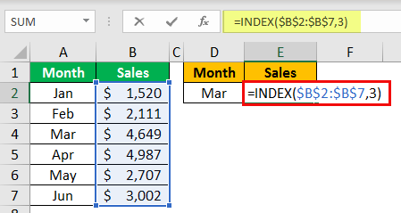
Step 4: That’s it! Close the bracket and press the "Enter" key. We will have sales value for the month of “Mar.”

Like this, based on the row number provided, we will get the value from the supplied array.
How To Use MATCH Function In Excel?
The MATCH function is used to find the lookup value position in the supplied array. In simple terms, lookup value row number or column number in the range of cells.
Example
For this example, consider the above data only.
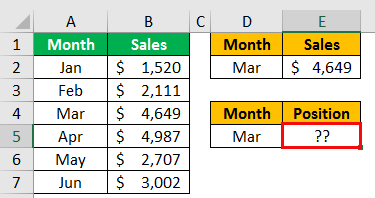
Step 1: From the above data, we are trying to get the month “Mar” position in cell E5. So, we must open the MATCH function in the E5 cell.
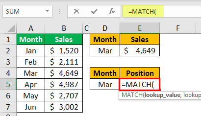
Step 2: The first argument is “lookup value,” so here, our lookup value is “Mar,” therefore, select the D5 cell.

Step 3: The lookup array is from which range of cells we are trying to look for the lookup value position. So, we must select the “Month” column.
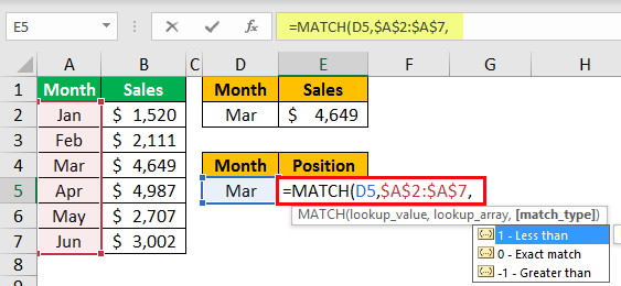
Step 4: The last argument is "MATCH type" since we look at the exact match supply 0.
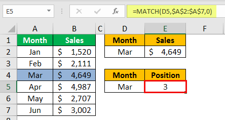
So, in the lookup array A2:A7, the position of the lookup value “Mar” is 3.
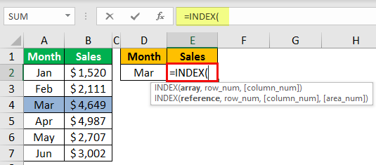
Combination Of INDEX + MATCH Function In Excel
The INDEX can return the result from the mentioned row number, and the MATCH function can give us the position of the lookup value in the array. Instead of supplying the row number to the INDEX formula, we can enclose the MATCH function to return the row number.
Example
Consider the below example.
Step 1: We must first open the INDEX function in cell E2.
Step 2: For the first argument, the array supplies B2 to B7.
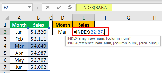
Step 3: Instead of supplying the row number as 3, open the MATCH function inside the INDEX function for the row number.
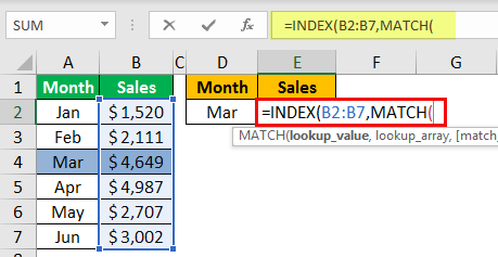
Step 4: Select the lookup value as a D2 cell.
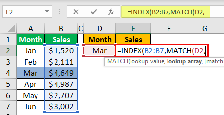
Step 5: Now, we must select the lookup array as A2 to A7.
Then, we must insert zero as the match type.
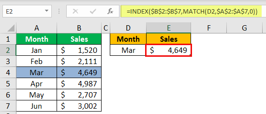
So, based on the row number provided by the MATCH function, the INDEX function will return the sales value. We can change the "Month" name in cell D2 to see dynamically changing sales value.
Powerful Alternative To VLOOKUP
We all have used the VLOOKUP function day in and day out. But, one of the limitations of VLOOKUP is that it can only fetch the value from left to right, not from right to left.
For example, look at the below data.
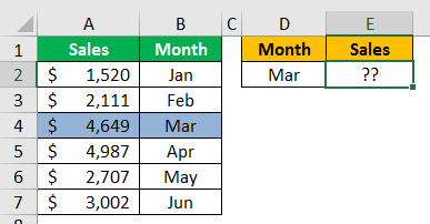
The above data lookup value is "Month," and the result column is "Sales." But, the data result column (Sales) is to the left of the lookup array table (Month), so we cannot use the Excel VLOOKUP function here, but we can still fetch with the combination of the INDEX function with the MATCH function for the data from the table.
Important Things To Note
- The INDEX function is used to obtain the result from row number.
- The MATCH function is used to find the position of the array value.
- Using the INDEX MATCH function, i.e., by combining the two functions in Excel, we can find better results than the VLOOKUP function.
