Table Of Contents
Combine Vlookup and Pivot Table in Excel
To use VLOOKUP in a PivotTable is similar to using the VLOOKUP function in any other data range or table:
- First, select the reference cell as the lookup value.
- Next, choose the data in the PivotTable for the table arguments array and then identify the column number with the output.
- Depending on the exact or close match, give the command and execute.
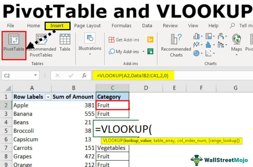
The PivotTable is one of the most powerful functions of Excel. A PivotTable is a table of statistics that helps to summarize and reorganize the data of a wide/broad table. This tool helps shorten the data and helps analyze the data categorize-wise and create a customized group. On the other hand, VLOOKUP is a function used in Excel when you are required to find things/values in data or range by row. This article looks at how to use VLOOKUP within the PivotTable.
VLOOKUP Excel Function - Explained in Video
How to use VLookup in Pivot Table Excel?
Let us follow the below steps.
Select the data on a worksheet for which you want to match the value from another worksheet. For example, deselect the category from the PivotTable. We will use the VLOOKUP here to get the category of product.
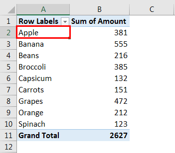
Suppose we want to get the category against each product. So, here we are using the VLOOKUP to get the data from another worksheet.The formula in the screenshot below searches for the text “Apple” in column B in the data worksheet.
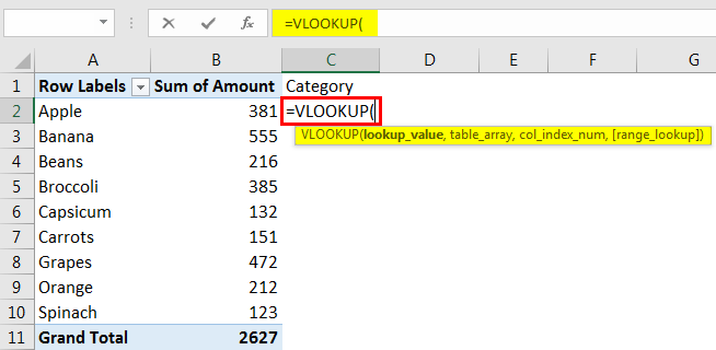
Enter the formula.
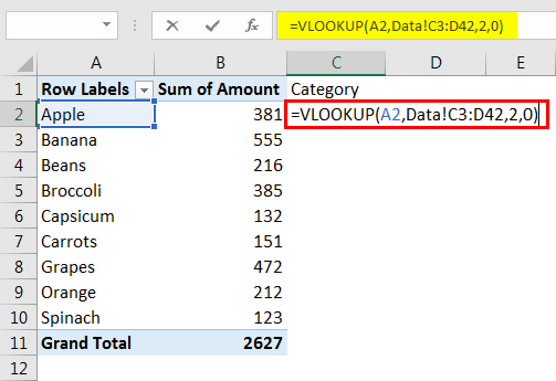
The formula looks for the value product “Apple,” in cell B5 from another worksheet.
Pivot Table’!C2:D42: We are getting the lookup value from sheet PivotTable against apple.
2,0 indicates that the value we are looking for a product is in column 2, and 0 means to find the exact match against each row.Press the "Enter" key to get the result.
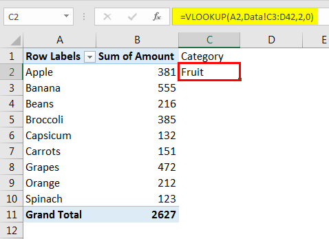
Drag the same formula against each product category.
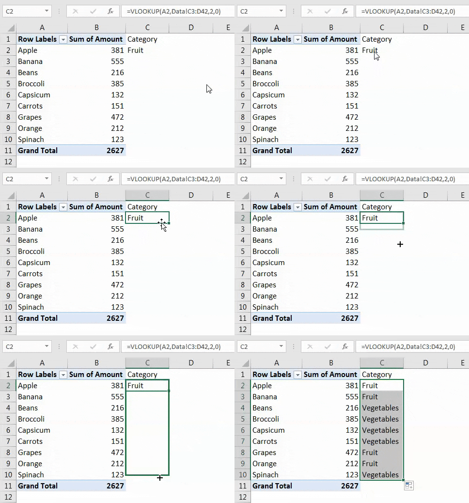
You will get the category against each product by using the formula VLOOKUP.
Things to Remember
- While creating a PivotTable, ensure there is no blank column or row.
- For the PivotTable, data should be in the right and correct form.
- We must Refresh the pivot table manually.
- In the PivotTable, always add the unique value in your column fields.
- We must always create a PivotTable in the new worksheet if you are a beginner or new user.
- We must summarize the data as much as possible to get better observation.
- VLOOKUP always searches for the value in the leftmost column of the lookup range.
- VLOOKUP is case insensitive.
- VLOOKUP can summarize or categorize the data in a very easy form.
- Once we use the VLookup formula, we must not shift the column or row. It leads to a mismatch of your VLOOKUP value.


