VLOOKUP To The Left

VLOOKUP to the left or reverse VLOOKUP is done to find the respective values in the reference cell's left column. Therefore, we cannot use it to reference the cells to the left of the reference cell. Still, we can create formulas to find the values to reference Excel's left. The INDEX and MATCH are such formulas that are combined. We can use conditional formulas in the LOOKUP function to find values to the left.

For example, we can find the VLOOKUP to the left in data as shown in the below image.

We can find the result by inserting the formula, =INDEX($A$2:$A$7,MATCH(G2,$B$2:$B$7,0)).

The result can be seen in the below image.

Let us learn VLOOKUP to the left in Excel in this article.

• VLOOKUP to the left or reverse VLOOKUP can be used to find the respective values in the reference cell's left column. Hence, it cannot be used to reference the cell to the left of the reference cell.
• INDEX and MATCH formulas can be used to locate values to the left. Even conditional formulas in the LOOKUP function can be used to search values located to the left.
• IF function and CHOOSE function in Excel in the VLOOKUP function can be nested for using the Reverse LOOKUP or VLOOKUP. They locate the values for a reference cell on the data table's left column.

For using the reverse lookup or VLOOKUP to the left, two functions can be nested in the VLOOKUP function to find the values for a reference cell on the left column of the data table. They are:

For using the reverse lookup or VLOOKUP to the left, two functions can be nested in the VLOOKUP function to find the values for a reference cell on the left column of the data table. They are:

1. If Function in Excel
2. Choose Function in Excel

In the above functions, we create an array data table and make Excel assume that the data on the left column is actually on the right column and find the exact match.

#1 - Using IF Function

Usually, in the VLOOKUP function, we search for values from left to right in a data table by the normal VLOOKUP function. It is impossible to search for a specific value from right to left. But in Excel, there are some tricks we can use to do that search. One such method is to use VLOOKUP with the IF function.

In the above formula, we have created an Excel array of two tables: ID and names. We are taking relative reference in excel of ID, searching them against the names from our array, and showing the exact match from the second column.

In the above formula, we are tricking Excel into believing that an A column is a second.

Method #2 - Using CHOOSE Function

Similar to what we did with the IF function, we can choose the function to find values using a LOOKUP function to the left of the data table. For the demonstration purpose, we will take the same data above and make some slight changes to the data. Have a look at the data below.

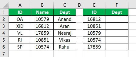
This time, we will find the department name concerning the ID provided.

In cell F2, write the following formula.

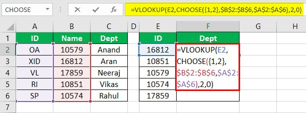
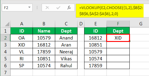
Again, we will explain the use of the function in detail below. But first, press the "Enter" key to watch the result.

Drag the formula to cell F6 and see the final result.

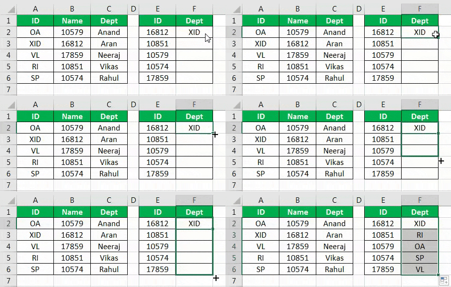
In the above example, we used the CHOOSE function nested in VLOOKUP to find the value on the right of the cell. Let me explain the choose function in detail:

• {1,2} This is the array created for the Data Table.
• We selected the data from the B column in the first column, which is our relative reference.
• In the second column, we chose the data from the A column, which is the data we want.
• In our formula, the "Name" column is the first column on the left, and the "ID" column is the second column on the right.
• Using the choose function, we used the VLOOKUP function to find the data from right to left.
• It is also known as the reverse lookup in excel.

#1 - Using Index Match Function

Consider the below table showing data of a musical shop with sample albums along with its price, genre and serial number.

Now, let us learn how to use INDEX function in Excel.

Step 1: First, we have to enter the INDEX function. Next, choose the Genre as array.

Step 2: Now, assume that we have to find the serial number, 318. Now, we should insert MATCH function.

Step 3: Now, assume that we have to find the serial number, 318. Now, we should insert MATCH function.

Next, enter G2, serial number as lookup value for MATCH function.

Step 4: Finally, we have to insert the table range, B2:B7 and enter 0 as exact match.

Step 5: Press Enter key. We can find the result as shown in the below image.

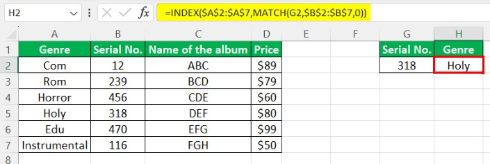
Likewise, we can use INDEX function to find VLOOKUP to the left.

#2 - Using XLOOKUP

Let us use the same example. Now, let us use XLOOKUP function to find the result corresponding to serial number, 116.

The steps are:

Step 1: Enter XLOOKUP function in cell H2.

Step 2: Enter the complete formula.

The formula is =XLOOKUP(G2,$B$2:$B$7,$A$2:$A$7)

We don’t have to insert MATCH function while using XLOOKUP function.

Step 3: Press Enter key.

We can find the result as shown in the above image.

Likewise, we can use XLOOKUP function to find VLOOKUP to the left.

This article is a guide to VLOOKUP to the Left in Excel. Here, we discuss using the VLOOKUP function from right to left in Excel using 1) IF function and 2) CHOOSE function, along with practical examples and a downloadable Excel template. You may learn more about Excel from the following articles: -

• VLOOKUP in Excel Pivot Table
• VLookup Function with IF
• VLOOKUP from Another Workbook
• VLOOKUP Errors