VLOOKUP Names

Last Updated :

21 Aug, 2024

Blog Author :

Edited by :

Reviewed by :

Table Of Contents

VLOOKUP Range Name

Names are "Named Ranges" for a range of Excel cells. We may need to fetch the data from a different worksheet. For choosing the table array, we must go to that particular sheet and select the range, which is time-consuming and frustrating. Have you ever faced a situation of working with ranges for applying the VLOOKUP formula? The answer is yes. Everybody faces tricky problems in selecting ranges for the VLOOKUP function. Often, we may choose the wrong range of cells, so it returns inaccurate results. In Excel, we have a way of dealing with these kinds of situations. This article will show you how to use "Names" in VLOOKUP.

Table of contents

VLOOKUP Range Name

Create a Named Range in Excel

Below are examples of names in VLOOKUP.

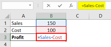
Look at the below formula in excel.

VLOOKUP Names Example 1.0

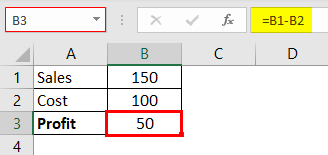
Profit (B3 cell) is determined using the formula B1 – B2. If any newcomer comes, they may not understand how profit arrives. Sales – Cost =Profit.

Instead of giving preference to the cell, how about the idea of giving the formula like the below one.

Example 1.1

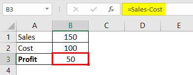
These are named ranges in excel. For example, we have named cell B1 as "Sales" and B2 as "Cost." So, instead of using cell addresses, we have used the names of these cells to arrive at the profit value.

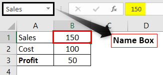
To name the cells, select cell B1 and give your name for this in this name box.

VLOOKUP Names Example 1.2

Similarly, do the same for the "Cost" cell as well.

Example 1.3

Now, we can use these names in the formula.

VLOOKUP Names Example 1.4

As you can see above, we have names of cell addresses instead of the cell address itself. We can notice the cell address by using the color of the names.

In the above example, Sales is in color Blue. Also, cell B1 has the same color. Similarly Cost color is red, and so is the B2 cell.

Learning Excel allows users to analyze complex data, automate tasks, and use advanced functions. Those looking to improve their data management skills using Excel can explore this Advanced Excel Functions Course.

VLOOKUP Excel Function - Explained in Video

How to Use Names in VLOOKUP?

Having learned about names and named ranges, let us see how we can use these in the VLOOKUP function.

Look at the below data set in excel.

Example 2

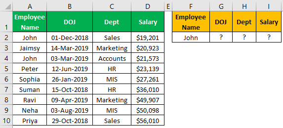
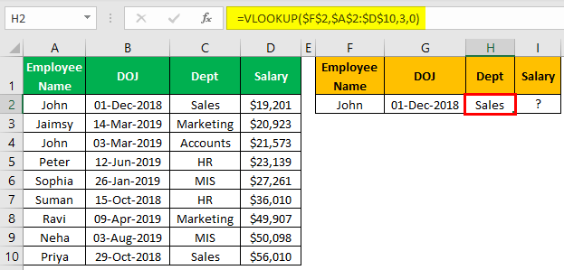
We have a data table from A1 to D10. It has employee information. On the other hand, we have one more table with only an employee's name. So, we need to fetch "DOJ," "Dept," and Salary" details using this employee's name.

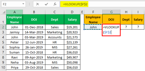
Open the VLOOKUP function and choose LOOKUP VALUE as an employee name.

VLOOKUP Names Example 2.1

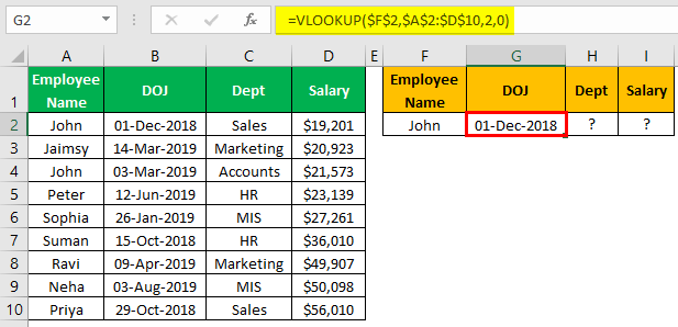
Choose the table array as a range of cells from A2 to D10 and make it an absolute lock.

Example 2.2

Now, mention the column number as 2 for "DOJ."

VLOOKUP Names Example 2.3

Mention column number 3 for "Dept."

Example 2.4

Mention column number 4 for "Salary."

VLOOKUP Names Example 2.12

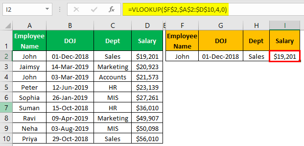
So, we have results here.

Now, using named ranges, we can not worry about choosing the range and making it an absolute reference.

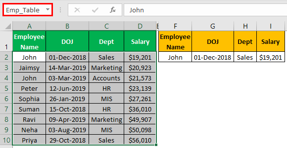
First, choose the table and name it "Emp_Table."

VLOOKUP Names Example 2.5.0

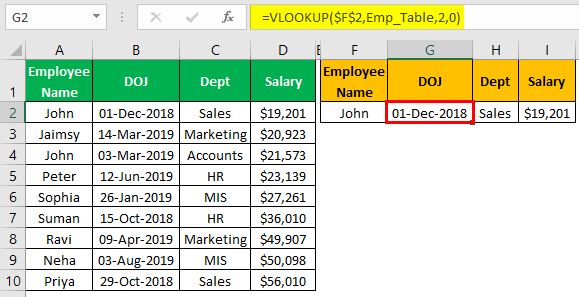
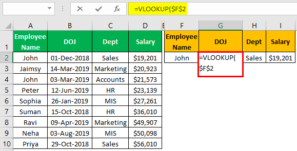
Again, open the VLOOKUP function, choose the lookup value as an F2 cell, and make it a column locked reference.

VLOOKUP Names Example 2.6.0

Now, we need to choose Table Array from A2 to D10 and make it an absolute reference. Instead, we will use the name given to this range, "Emp_Table."

VLOOKUP Names Example 2.7.0

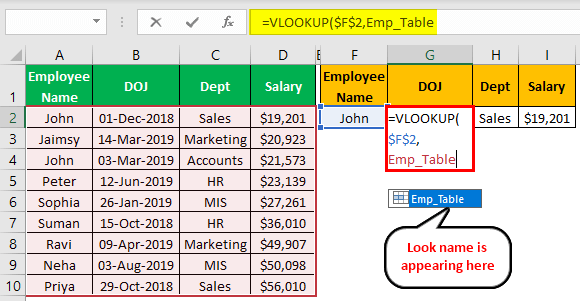
As you can see above, as soon as we selected the named range, it highlighted the referenced range with the same color as the name.

Now, mention the column index number and range lookup type to get the result.

VLOOKUP Names Example 2.8.0

So, using this named range, we need to worry about selecting the table array now and then and making it an absolute reference.

VLOOKUP Named Range List and Editing

Once the named ranges are created, we can find all the named ranges of the workbook under the FORMULAS tab and Name Manager.

VLOOKUP Names Example 2.9.0

Click on this, and we may see all the named ranges here.

Example 2.10

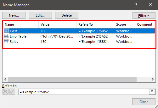
Choose any names and click on "Edit" to see their actual cell references.

VLOOKUP Names Example 2.11.0

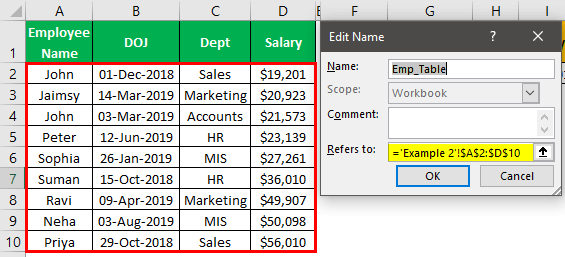
The "Emp_Table" named range is referenced from A2 to D10.

Things to Remember Here

The named ranges are useful when regularly applying the VLOOKUP formula. Also, it is very helpful if we need to go to different worksheets to select the table array.
While naming the range, we cannot include any special characters except underscore (_), we cannot include space, and the name should not start with a numerical value.