Table Of Contents
Combine VLOOKUP with Match
The VLOOKUP formula is the most commonly used function to search and return either the same value in the specified column index or the value from a different column index concerning the matched value from the first column. The major challenge faced while using VLOOKUP is that the column index to be specified is static and does not have dynamic functionality. Especially when you are working on multiple criteria that require you to change the reference column index manually, this need is fulfilled by using the “MATCH” formula to have a better grip or control of the frequently changing column index in the VLOOKUP formula.
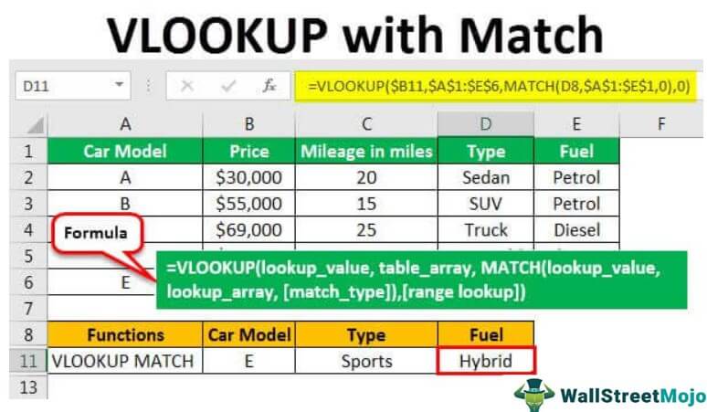
VLookup and Match Formula
#1 - VLOOKUP Formula
The formula of the VLOOKUP function in Excel:

Here, all the arguments to be entered are mandatory.
- lookup_value – Here, a reference cell or text with double quotes should be entered to be identified in the column range.
- table_array – This argument requires the table range to be entered where the lookup_value should be searched and the data to be retrieved resides in the particular column range.
- col_index_num – In this argument, the column index number or the count of the column from the reference first column needs to be entered from which the corresponding value needs to be pulled from the same position as the value searched in the first column.
- – This argument will give two options.
- TRUE – Approximate match:- The argument can either be entered as “TRUE” or numeric “1”, which returns the approximate match corresponding to the reference column or first column. Moreover, we must sort values in the first column of the table array in ascending order.
- FALSE – Exact match:- Here, the argument to be entered can either be “FALSE” or numeric “0”. This option will only return the exact match of the value corresponding to be identified from the position in the first column range. Failure to search the value from the first column would return a #N/A error message.
#2 - Match Formula

The MATCH function returns the cell position of the value entered for the table array.
All the arguments within the syntax are mandatory.
- lookup_value – The argument entered can be either the cell reference of the value or a text string with double quotes whose cell position is required to be pulled.
- lookup_array – The table array range must be entered whose value or cell content is desired to be identified.
- – This argument provides three options, as explained below.
- “1-Less than” – The argument to be entered is numeric “1,” which will return the value that is less than or equal to the lookup value. And also, we must sort the lookup array in ascending order.
- “0-Exact match” – The argument to be entered should be numeric “0”. This option will return the exact position of the matched lookup value. However, the lookup array can be in any order.
- “-1-Greater than” – The argument to be entered should be numeric “-1”. The third option finds the smallest value greater than or equal to the lookup_value. Here, we must place the order for the lookup array in descending order.
#3 - VLOOKUP with MATCH Formula
=VLOOKUP(lookup_value, table_array, MATCH(lookup_value, lookup_array, ),)
How to Use VLOOKUP with Match Formula in Excel?
The example below will help understand the functioning of the VLOOKUP and MATCH formula when put together.
Consider the below data table, which describes the specifications of the given vehicle to be purchased.
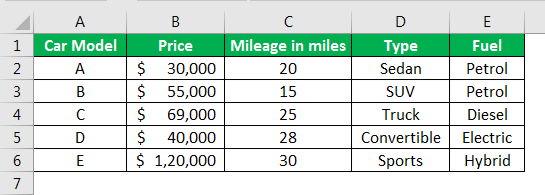
To clarify the combined function for the VLOOKUP and MATCH function, let us understand how the individual formula operates and then arrive at the VLOOKUP MATCH results when put together.
Step #1 - Let us apply the VLOOKUP formula at an individual level to arrive at the result.
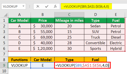
The output is shown below:
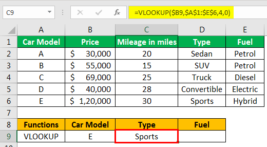
Here, the lookup_value is referred to as $B9, is model “E,” and the lookup_array is given as the range of the data table with absolute value “$” the column_index is referred to as column “4,” which is the count for column “Type,” and the range lookup is given an exact match.
Thus, the following formula is applied for returning the value for column “Fuel.”

The output is shown below:
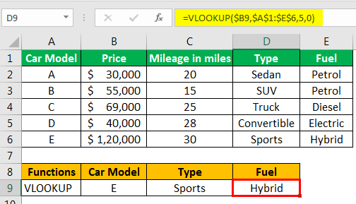
Here, the lookup_value with absolute string “$” applied for lookup value and lookup_array helps fix the reference cell even if the formula is copied to a different cell. For example, in the “Fuel” column, we need to change the column index to “5” as the value from which the data required to be retrieved changes.
Step #2 - Now, let us apply the MATCH formula to retrieve the position for the given lookup_value.
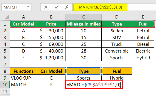
The output is shown below:
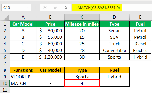
As the above screenshot shows, we are trying to retrieve the column position from the table array. In this case, the column number to be pulled is called cell C8, column “Type,” and the lookup_range to be searched is given as the range of column headers, and the match type is given an exact match to be as “0”.
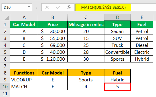
Thus, the below table will give the desired result for the positions of column “Fuel.”

Here, the column searched is given to be cell D8, and the desired column_index is returned to be “5”.
Step #3 - We will use the MATCH formula within the VLOOKUP function to get the value from the identified column position.
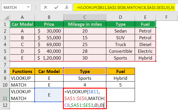
The output is shown below:
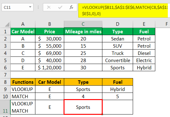
In the above formula, the MATCH function is put in place of the column_index parameter of the VLOOKUP function. Here, the MATCH function will identify the lookup_value reference cell “C8” and return the column number through the table array. This column position will serve as an input to the column index argument in the VLOOKUP function. Which, in turn, will help VLOOKUP identify the value returned from the resultant column index number?
Similarly, we have also applied VLOOKUP with a MATCH formula for the “Fuel” column.
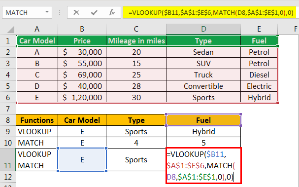
The output is shown below:

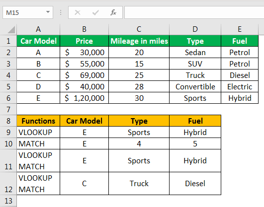
We can thereby apply this combination function for other columns “Type” and “Fuel” as well.
Things to Remember
- We can apply VLOOKUP to lookup values only on its foremost left-hand side. Any values present to be searched on the right side of the data table will return the #N/A error value.
- The range of table_array entered in the second argument should be absolute cell reference “$” because it will maintain the fixed table array range when applying the lookup formula to other cells. Otherwise, the table_array, range reference cells will shift to the next cell reference.
- The value entered in the lookup_value should not be smaller than the smallest value in the first column of the table array. Else, the function will return the #N/A error value.
- Before applying an approximate match “TRUE” or “1” in the last argument, we must always remember to sort the table array in ascending order.
- The MATCH function only returns the position of the value in the vlookup table array and does not return the value.
- If the MATCH function cannot identify the position of the lookup_value in the table array, then the formula returns #N/A in the error value.
- VLOOKUP and MATCH functions are case insensitive when matching the lookup_value with the matching text value in the table_array.


