What Is Dynamic Tables In Excel?
Dynamic Tables in Excel are the tables where we add, or update new values in an existing dataset. As a result, the table readjusts itself w.r.t the size, also refreshing or modifying the linked generated reports and PivotTables with the changes in the datset.
We can create Excel Dynamic Tables with two different methods: making a table of the data from the Table section, and another using the OFFSET function.
Key Takeaways
- Dynamic means a process or system characterized by a constant change or change in any activity.
- The Dynamic Tables in Excel make any dataset dynamic so that the linked PivotTables, the linked referenced formulas, update dynamically with the slightest modifications.
- Rarely, we might have to refresh the pivot table manually, but not always, because any changes or modifications will automatically reflect in the formula results.
- Using the OFFSET function, we can create dynamic named ranges. We can also use the COUNTA with the OFFSET function to count the data in columns.
How To Create Dynamic Tables In Excel?
There are two basic ways of using Dynamic Tables in Excel –
- Using TABLES.
- Using the OFFSET function.
Examples
We will consider examples to create Dynamic Tables in Excel using the above-mentioned methods.
Example #1 – Using Tables to create Dynamic Tables in Excel
Using tables, we can build a Dynamic Table in Excel and base a pivot over the Dynamic Table.
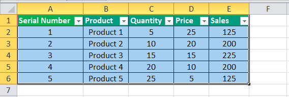
We have the following data,
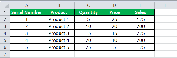
When we create a pivot table with this data range from A1:E6, and then insert new data in dataset row 7, it will not reflect in the PivotTable.
So, we will first make a dynamic range. The steps are,
- We must first select the data, A1:E6.

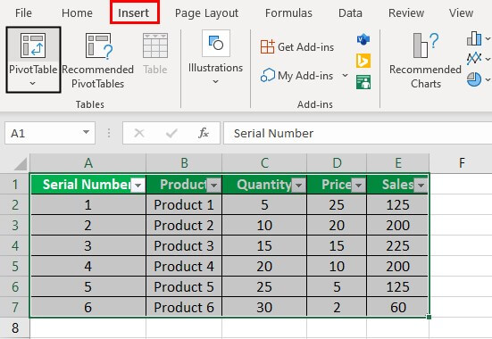
- Now, in the “Insert” tab, we must click the “Table” under the “Tables” section.

- Next, we have to select the data. Then, in the “Insert” tab under the Excel “Tables” section, click on “PivotTable.”
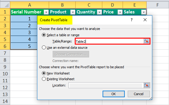
- As a result, a dialog box will pop up, as shown below, then click “OK.”
- As our data has headers, we must remember to check the box “My table has headers” and click “OK.”
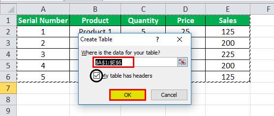
- Now, our dynamic range is created.
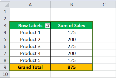
- As we have created the table, it takes a range as Table 2. Click on “OK,” and in the “PivotTable,” drag “Product” in rows and “Sales” in values.
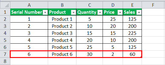
- In the sheet where we have our table, we must insert another piece of data on the 7th.
Refresh the pivot table.Our dynamic PivotTable has automatically updated the “Product 6” data in the PivotTable.
Example #2 – Using the OFFSET Function to create a Dynamic Table in Excel
We can also use the OFFSET Function to create Dynamic Tables in Excel. Let us have a look at one such example.
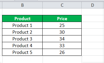
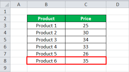
We have a price list for the products we use for our calculations.
First, we must select the data and give it a name.
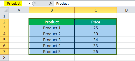
Whenever we refer to the data set price list, it will take us to the data in the range B2:C7, which has our price list. But if we update another row to the data, it will still take me to the range of B2:C7 because our list is static.
The steps to use the OFFSET function to make the data range dynamic are,
#1 – Now, under the “Formulas” tab in the “Defined Range,” we must click on “Define Name”.
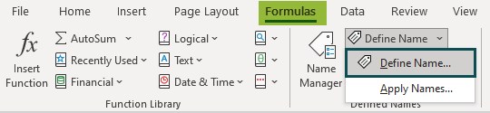
The “New Name” dialog box will pop up.
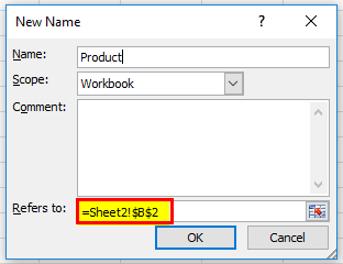
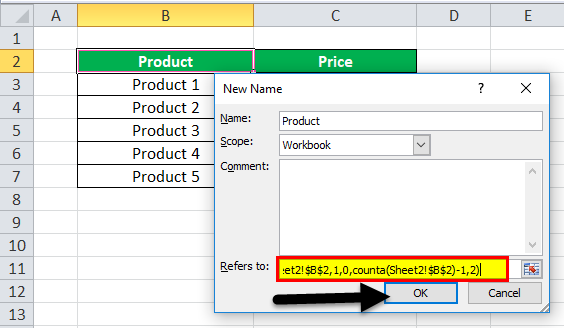
#2 – We can type any name in the Name Box. We will use the “Product.” The scope is the current workbook, which refers to the current selected cell B2.
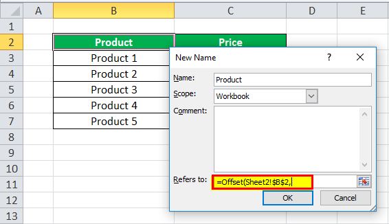
In “Refers to”, we must write the following formula:
=offset(Sheet2!$B$2,1,0,counta(Sheet2!$B:$B)-1,2)
=offset(
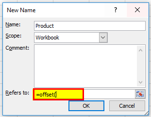
#3 – Now, we must select the starting cell, which is B2.
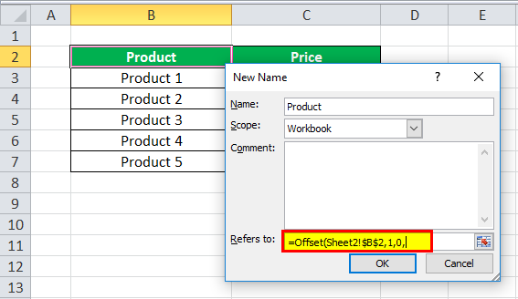
#4 – Now, we must type 1,0 as it will count how many rows or columns to go.
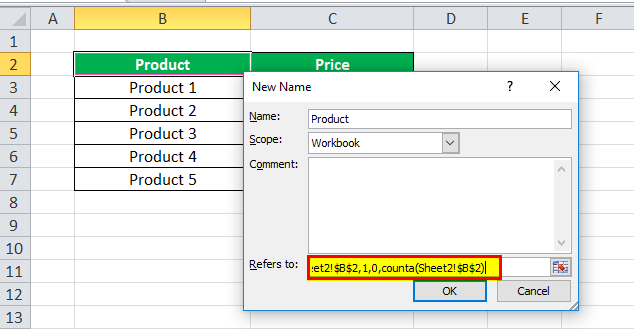
#5 – Now, we need it to count the data in column B and use that as the number of rows so that we may use the COUNTA function and select column B.
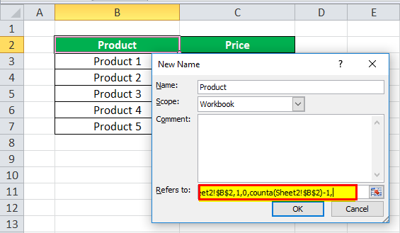
#6 – As we do not want the first row, the product header, to be counted, so (-) 1 from it.
#7 – Now, the number of columns will always be two, so we must type “2” and click “OK.”
#8 –This data range would not be visible by default, so to see this, we must click on Name Manager under the “Formula” tab and select “Product.”
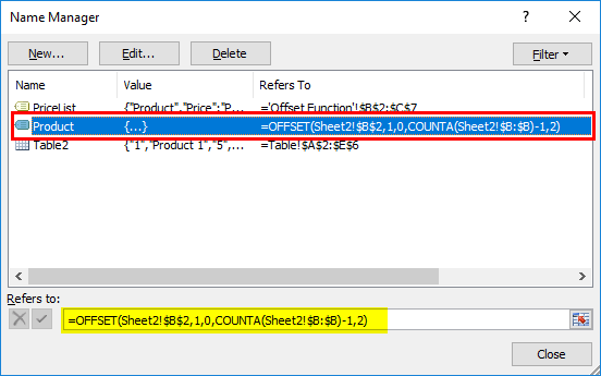
#9 – If we click on “Refers to,” it shows the data range,

#10 – We will add another product -“Product 6.”
#11 – Lastly, click on “Product Table” in the “Name Manager.” It also refers to the new data inserted.

Like this, we can use the OFFSET function to make Dynamic Tables.
Important Things To Note
- The PivotTables based on dynamic range automatically gets updated when refreshed.
- Using the OFFSET function in “Defined Name” can be seen from the “Name Manager” in the “Formula” tab.
Frequently Asked Questions (FAQs)
What are the advantages of Dynamic Tables in Excel?
The advantages of Dynamic Tables in Excel are,
- In Excel when we create lists or data in a workbook and make a report out of it. But if we add, remove, move, or change the data, then the whole report can be inaccurate. Dynamic Tables help us with the same because whenever a list or data range is updated or modified, it ensures that it will change the report as per the data change.
- A dynamic range will automatically expand or contract as per the data change.
- The PivotTables based on the Dynamic Table in Excel can be automatically updated when the pivot is refreshed.
What is the difference between a Dynamic Table in Excel and a Static Table?
As we considered in the article above, the Dynamic Tables take a structured reference, however, the Static Tables take cells or a cell range as a reference.
Why is the Dynamic Table in Excel not working?
The Dynamic Table in Excel may not work for the following reasons,
- The generated PivotTable did not get automatically refreshed once the data was modified in the dataset. Then, we can manually refresh the PivotTable.
- The named range table might be deleted or renamed. Ensure to keep the right Table linked throughout.
Recommended Articles
This article is a guide to Dynamic Tables in Excel. Here we generate PivotTables for dataset that updates when data is modified, OFFSET(), examples, Template. You may learn more about Excel from the following articles: –