How to Find Duplicates in Excel?
In MS Excel, the duplicate values can be found and removed from a data set. Depending on your data and requirement, the most commonly used methods are the conditional formatting feature or the COUNTIF formula to find and highlight the duplicates for a specific number of occurences. The columns of the data set can be then filtered to view the duplicate values.
In this article, we will look at 5 different methods to check, identify, and delete duplicates in Excel.
5 Methods to Check & Identify Duplicates in Excel
#1 – Conditional Formatting
The conditional formatting feature is available in Excel 2007 and subsequent versions.
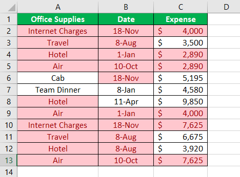
The following table consists of the expenses incurred on availing certain office facilities. The corresponding dates of purchasing such facility are also listed.
We want to identify the duplicates in excel with the help of conditional formatting.

The steps to find the duplicates in excel with the help of conditional formatting are listed as follows:
- Select the data range (A1:C13) where duplicates are to be found.
- In the Home tab, select “conditional formatting” from the “styles” section. From the drop-down menu, select “highlight cell rules” and click on “duplicate values.”

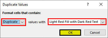
- The pop-up window titled “duplicate values” appears. In the first box on the left side, select “duplicate.” In the “values with” drop-down, select the required color to highlight the duplicate cells. Click “Ok.”

- The duplicate cells are highlighted in the data table, as shown in the following image.

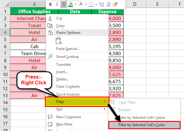
- The columns can be filtered to identify the duplicate values. For this, right-click the required column and select “filter by selected cell’s color.” The data is filtered for duplicates.

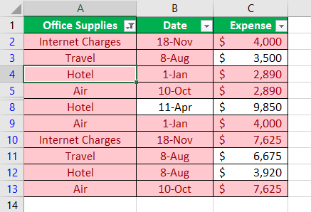
- The result after applying the filter to the first column (office supplies) is shown in the following image.


#2 – Conditional Formatting (Specific Occurrence)
Let us consider an example to identify the specific number of duplications. In the following table, we want to check and show the duplicate values with three occurrences.

The steps to find the duplicate values for specific number of occurrences are listed as follows:
Step 1: Select the range A2:C8 in the given data table.
Step 2: In the Home tab, select “conditional formatting” from the “styles” section. Click “new rule.”

Note: The “new rule” option helps highlight a specific count of duplicates using the COUNTIF formula.
Step 3: The pop-up window titled “new formatting rule” appears. Enter the following details, as shown in the succeeding image.
- Under “select a rule type,” select “use a formula to determine which cells to format.”
- Under “edit the rule description,” enter the COUNTIF formula.
The COUNTIF formula “=COUNTIF(cell range of the data table, cell criteria)” finds and highlights the cells for the desired number of occurrences.
In this case, the COUNTIF formula highlights duplicate cells having triplicate count. This count can be changed to a greater number. The conditions can also be changed depending on the user’s requirement.
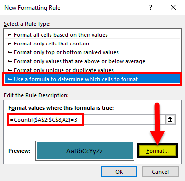
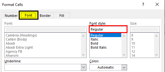
Step 4: Once the COUNTIF formula is entered, click “format.” The pop-up window titled “format cells” opens. Select the font style “regular.”
Step 5: In the “fill” tab, select blue color. The “fill” tab helps highlight the duplicate cells.
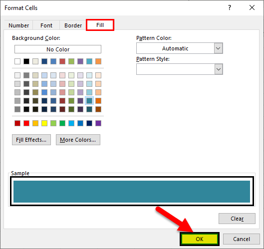
Step 6: Once the selections in “format cells” window are complete, click “Ok.” Click “Ok” again in the “new formatting rule” window.
Step 7: The result is displayed in the following image. The duplicate cells with three occurrences are highlighted.

#3 – Change Rules (Formulas)
Working on the data of example #2, let us understand the procedure of changing the formula. For applying new formulas, the existing rules (formulas) of the data table have to be cleared.
The steps to clear the existing rules (shown in the succeeding image) are listed as follows:
Step 1: In the Home tab, select “conditional formatting” from the “styles” section.
Step 2: In “clear rules” option, select either of the following:
- Clear rules from selected cells–This resets the rules for the selected range of the table. So, prior to clearing the rules, the data needs to be selected.
- Clear rules from entire sheet–This clears the rules for the entire sheet.
The blue highlighted cells disappear and the original table is displayed.

#4 – Remove Duplicates
Let us check and delete duplicate values from a selected range. Prior to deletion, keeping a copy of the table is advisable because the duplicates will be permanently deleted.
The following table displays a series of items with their corresponding IDs.

The steps to find and delete duplicate values are listed as follows:
Step 1: Select the range of the table whose duplicates are required to be deleted.
Step 2: In the Data tab, select “remove duplicates” from the “data tools” section.

Note: The “remove duplicates” option helps eliminate duplicates and retain unique cell values.
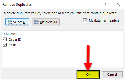
Step 3: The pop-up window titled “remove duplicates” appears, as shown in the succeeding image. By default, the following options are already selected:
- The checkboxes for both the headers (“order ID” and “items”)
- The “select all” box
Since the table consists of column headers, select the checkbox “my data has headers.” Click “Ok” to execute.
Note: To change the number of columns selected, click “unselect all.” Following this, the desired columns from which the duplicates are to be deleted can be selected.
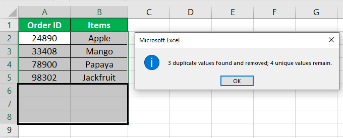
Step 4: The result is shown in the succeeding image. A prompt is displayed which states the following details:
- The number of duplicate values removed from the table
- The number of unique values that remain in the table after deletion
Click “Ok.” Hence, the duplicate values along with their corresponding rows are deleted.
#5 – COUNTIF Formula
The following table displays the names of a few countries. We want to identify the duplicate values using the COUNTIF function.
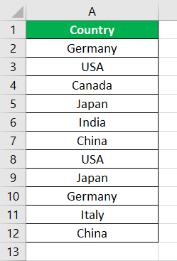
The COUNTIF function requires the range (column containing duplicate entries) and the cell criteria. It returns the number of corresponding duplicates for every cell.
The steps to find the duplicate values in excel with the help of the COUNTIF function are listed as follows:
Step 1: Enter the formula shown in the succeeding image. Press the “Enter” key.
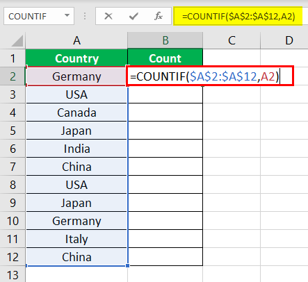
Note: The range must be fixed with the dollar ($) sign. Otherwise, the cell reference will change on dragging the formula.
Step 2: Drag the formula till the end of the table with the help of the fill handle. Alternatively, place the cursor on cell B2 and double-click the fill handle. The fill handle appears at the lower right corner of cell B2.
Step 3: The output of the formula is shown in the following image. It returns the count of duplicates for the entire data set.

Note: The filter can be applied to the column header to view the occurrences greater than one.
Frequently Asked Questions (FAQs)
What does it mean to find duplicates in Excel?
While consolidating different worksheets, several duplicates may be found in a data set. MS Excel helps to find and highlight such duplicates. It is also possible to filter a column for duplicate values.
An easy way to search for duplicates is by using the COUNTIF formula. This formula can count the total number of duplicates in a column. It can also count the number of individual instances of a particular duplicate entry. It accepts two arguments–the range and the criteria.
How to find duplicates in a column of Excel?
To check a column for duplicates, the formula is given as follows:
“=COUNTIF(A:A,A2)>1”
The formula checks for duplicates in column A. The topmost cell is A2. For every duplicate value, the formula returns “true.” For every unique value, the formula returns “false.”
Note: For an output other than “true” and “false,” the COUNTIF formula can be enclosed in the IF function.
What is the formula to find duplicates in Excel?
The generic formula to find the exact, case-sensitive duplicate values is stated as follows:
“IF(SUM((-EXACT(range,uppermost_cell)))<=1,””,”Duplicate”)”
The EXACT function compares the cell range with the target cell. The SUM function adds the number of instances. If the occurrence is greater than 1, the IF function returns “duplicate.”
Note 1: Since it is an array formula, it should be entered using “Ctrl+Shift+Enter.”
Note 2: If the same word appears twice in lowercase and once in uppercase, the formula will not count the uppercase word as duplicate.
Recommended Articles
This has been a guide to Find Duplicates in Excel. Here we discuss how to identify, check and show duplicates in excel with examples. You may also look at these useful functions in Excel –