Group Data In Excel

Group data in Excel, as the name suggests, combines data into a group. The more data you have, the more confusion it will create in the final summary sheet. For example, if we show monthly sales reports from different categories and if the categories are too many, then we cannot see the full view of the summary in a single window frame. When the summary exceeds more than one window frame, we need to scroll down or scroll across to see the other month’s numbers. So in such cases, it is a good idea to group the data.

Too many subcategory line items may be overwhelming and complex to read. It increases the chances of reading wrongly. The good thing is that Excel is flexible, and we can organize the data in the group to create a precise summary by adding PLUS or MINUS signs.

In this article, we will show you the ways of grouping data in Excel.

Grouping data helps us analyze and manage data with ease. Let us learn how to group data in Excel with detailed examples.

Example #1

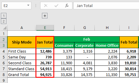
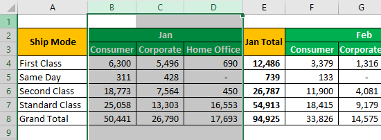
Below is the summary of the monthly sales summary across different business categories.

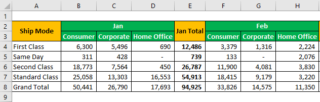
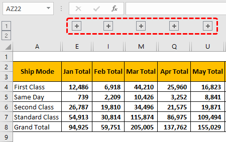
As we can see above, we could see only two monthly summaries in the single page view. To see other months' summaries, we need to scroll to the right side of the sheet. But by grouping the data, we can see it in a single page view like the one below.

Let us show you how to group the first-month sub-category breakup.

• Step 1: We must select columns that we need to group. In this example, we need to group subcategory breakup columns and see the monthly total, so we need to choose only subcategory columns.

• Step 2: After selecting the columns for the group, we must next go to the "Data" tab. Under the "Outline" category of the "Data" tab, we have a "Group" option.

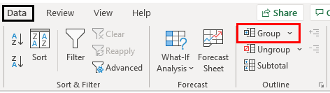
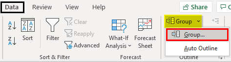
• Step 3: Click on the drop-down list in Excel of "Group" and again choose "Group."

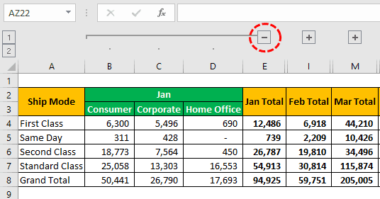
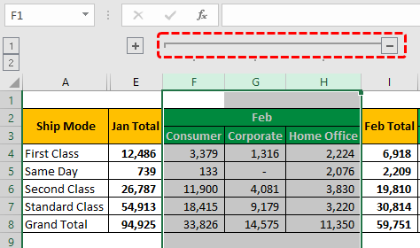
As soon as we select the "Group" option, we can see the grouped columns.

Then, we must Click on the "minus" icon to see only the "Jan" month total.

• Step 4: Similarly, we must select the second month "Feb" columns and group the data.

• Step 5: One tip here is that we need not click on the "Group" option from the "DATA" tab. Rather, once the first-month grouping is over, select the second-month column and press the F4 key to repeat the previous task.

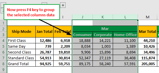
Like this, we can repeat the steps for each month to group the data.

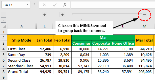
So, whenever we want to see the particular month sub-category breakup, we need to click on the "PLUS" icon to expand the grouped columns view.

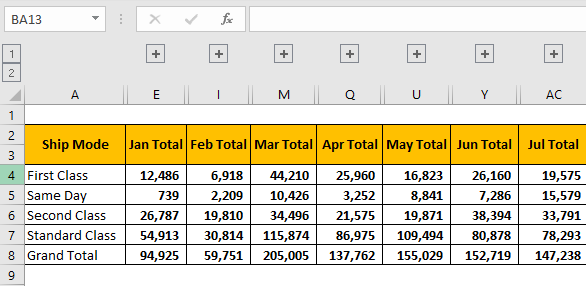
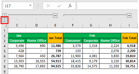
For example, if we want to see "Mar" month subcategory breakup values, we must click on the "PLUS" icon.

To group the columns, click on the  "MINUS" sign.

Example #2 - Shortcut Key To Group The Data

A shortcut is a way of increasing the productivity in excel, so grouping the data to have a shortcut key.

The shortcut key to the group selected data is ALT + SHIFT + Right Arrow.

• Step 1: First, we must select the columns to be grouped.

• Step 2: Now press the shortcut key ALT + SHIFT + Right Arrow.

Example #3 - View Collapsed (Expanded) And Grouped Data Quickly

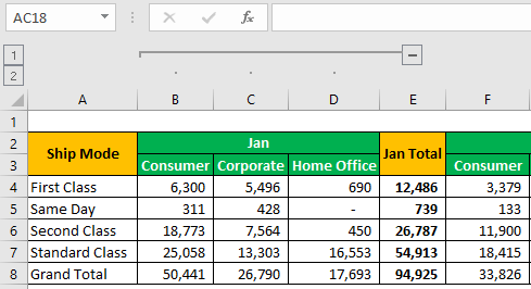
We can group the data to view a single-page summary or single window frame summary in Excel as we did above. We see level buttons when we group the data at the top left of the worksheet.

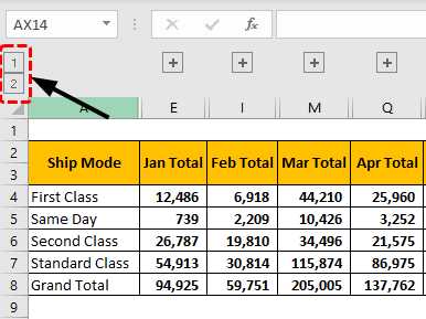
If we click on the first level button, "1," we can see "grouped" data. When we click on the level button "2," we can see "expanded" data.

• Grouping is the way of showing only the main data.
• While grouping the Excel data, we must select all the data columns we need to group and leave out the column to be seen.
• The shortcut key to group the selected data columns is ALT + SHIFT + Right Arrow.