What Is Highlight Duplicate Values In Excel?
A duplicate value occurs more than once in a dataset. It is often found while working with large databases in excel. It is essential to find and highlight the duplicate values in excel because the user may or may not want to retain them.
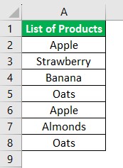
For example, consider the below table with the list of products. Now, let us highlight duplicate values in Excel.
The steps are:
Step 1: First, we need to select the cell range.
Step 2: Next, select Home > Conditional Formatting under Styles group.
Step 3: Then, choose Highlight Cells Rules > Duplicate Values… option.
The Duplicate Values window opens.
Step 4: Now, choose the desired color and then, click OK.
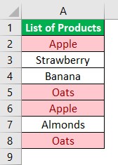
Likewise, we can highlight duplicate values in Excel with ease.
Key Takeaways
- Highlight Duplicate values in Excel is a built-in function used to highlight values.
- The shortcut to highlight duplicate values in Excel are Alt+H+L+H+D.
- Remember, the purpose of highlighting duplicates in excel is to make the data understandable and accurate.
- Moreover, it helps in differentiating the unique values from the duplicated ones.
- We can highlight duplicate values from multiple columns in Excel.
- Similarly, we can remove the duplicate values in Excel by selecting the cell range and clicking on Data > Remove Duplicates option.
How To Highlight Duplicate Values In Excel?
We can highlight the duplicate values in a single excel column as well as in an entire worksheet. The difference between the former and the latter is in the selection of cells. Hence, one must be careful while selecting cells in the first step.
Let us consider a few examples.
Examples
Example #1 – Highlight Current Duplicates In The Selected Excel Range
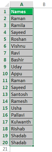
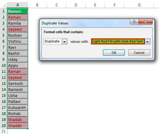
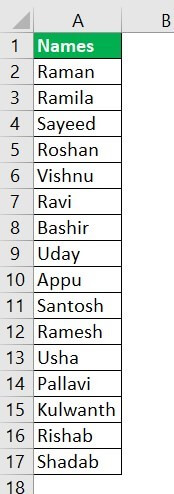
The following table shows the list of names of a few people. We want to find and highlight the current duplicates with the help of conditional formatting.
The steps are:
- To begin with, select the data range that consists of the duplicate values.Note:In this case, ensure that only the particular range containing duplicates is selected and not the entire worksheet.

- Next, click theconditional formattingdrop-down under the “styles” group of the Home tab. In “highlight cells rules,” select duplicate values, as shown in the following image.
Alternatively, press theshortcutkeys “Alt+H+L+H+D” one by one.

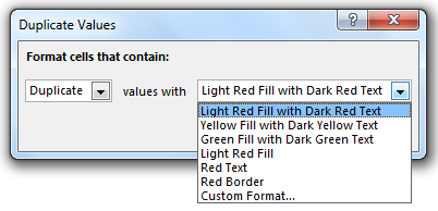
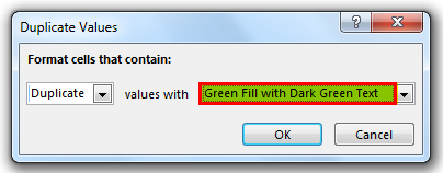
- Then, the “duplicate values” dialog box opens, as shown in the following image. One can choose the requiredtype of formattingin the “values with” box.It is possible to highlight either the cell, the text or both with different colors. One can also highlight the borders of the cells containing duplicates.

- Now, select “light red fill with dark red text” and click “Ok.” The values appearing more than once in the selected range (column A) are highlighted, as shown in the following image.


Example #2–Highlight Future Duplicates In The Selected Range
The table consists of the invoice numbers and amounts. Now, we want to perform both the following tasks:
- Highlight the current duplicate values
- Highlight the duplicate values to be entered in the future
The steps are:
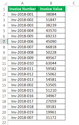
Step 1: To start with, select the column “invoice number” (column A). With this selection, it will be possible to highlight the new duplicate value entered in the existing list (column A) in future.
Step 2: Next, in the Home tab, click the conditional formatting under the “styles” group. Select “duplicate values” from “highlight cells rules,” as shown in the following image.
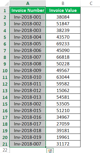
Step 3: Then, we need to select the color. Let us select “green fill with dark green text.” Click “Ok.”
Step 4: As we can see, the duplicate values are highlighted. These are the ones that are occurring more than once.

Step 5: Now, enter any of the duplicate invoice numbers in row 22 of column A. Automatically, the new duplicate entry of column A is highlighted.
Note 1: Alternatively, select the entire worksheet (in step 1) and perform the steps 2 and 3. The results will be the same as those obtained in step 4.
Note 2: There is a difference between selecting a specific column and the worksheet. In the former, the duplicate value entered in a new cell of the same column will be highlighted. In contrast, the duplicate value entered in any cell of this worksheet will be highlighted.

Example #3–Remove Duplicates From The Selected Range
Working on the data of example #1, we want to remove the duplicates from the selected range.
The steps are:
Step 1: To begin with, select the data range containing duplicates.
Step 2: Next, click “remove duplicates” from the “data tools” group of the Data tab.
Alternatively, press the shortcut keys “Alt+A+M” one by one.

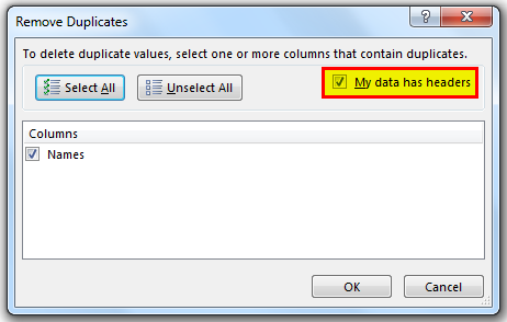
Step 3: Now, the “remove duplicates” dialog box appears, as shown in the following image. The box under “columns” shows the header of the chosen column.
Next, select “my data has headers.” Click “Ok.”
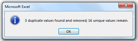
Step 4: The duplicate values are removed from the selected column (column A). A message appears stating the number of duplicates deleted and the number of unique values retained.
Click “Ok” to see the results.
Step 5: The column A now shows only the unique data values. Hence, the duplicate values have been removed.
The Cautions Governing Duplicate Values
- First, we need to make sure to select the correct range to highlight the duplicates.
- Ensure that you select the “custom format” option in the “duplicate values” dialog box to choose the formatting style of the duplicate cells.
- Remember to select the correct column header while removing the duplicates.
Important Things To Note
- Highlight Duplicate values identifies the duplicate values in Excel worksheet.
- Prior to deleting the duplicates permanently, it is recommended to keep a copy of the original data.
- This allows one to return to the source data, if required.
Frequently Asked Questions (FAQs)
What does highlight duplicates in Excel mean?
Highlighting same or duplicated values allows users to review every duplicate value and decide whether to retain or remove it.
Explain how to highlight duplicates in Excel with an example.
Consider the below table with the list of students and the marks obtained by them. Now, let us find the duplicate values using highlight duplicate values in Excel.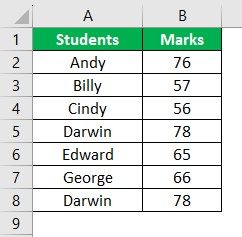
Step 1: To start with, select the cell range A1:B8.
Step 2: Then, select Home – Conditional Formatting under Style group.
Step 3: Now, choose Highlight Cells Rules – Duplicate Values… option.
The Duplicate Values window opens.
Step 4: Choose the desired color and click OK.
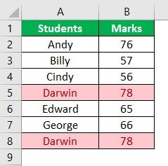
Likewise, we can highlight duplicate values in Excel with ease.
How to highlight duplicates in multiple columns with an Excel formula?
a. Select the entire range.
b. Click the Conditional Formatting > Home tab. Select New Rule.
c. The New Formatting Rule window opens. Choose Use a formula to determine which cells to format under Select a rule type.
d. Under Edit the rule description, enter the formula, =COUNTIF(range,top_cell)>1
e. Click Format and select OK.
f. Click OK again in the New Formatting Rule window.
Likewise, we can highlight duplicates in multiple columns with Excel formula.
Recommended Articles
This has been a guide to guide to Highlight Duplicates in Excel. Here we discuss how to find and highlight duplicate values in excel with step by step examples You may learn more about Excel from the following articles-