Power Query Tutorial

Power Query is a versatile tool that makes solving common tasks related to data much simpler. It helps save time spent on manual tasks like combining cells, cut, copy and paste, etc. Using the Power Query tool makes it a lot easier to perform such tasks. 

In this Power Query tutorial, we see how the tool can be used to solve manual tasks with ease. It is a comprehensive guide to master Power Query to enhance efficiency and date workflow. 

Working with Excel Power Query is just fun because of its user-friendly options. It has so many features which we will explain with examples. .

From Excel 2016 onwards, it is a built-in tool available in the Get & Transform Data Section under the Data Tab. 

In earlier versions of Excel 2013 and 2010, it is available as a free add-in which can be downloaded from Microsoft’s website. 

Example - Import Data from Text File

Step-by-Step Example to Import Data

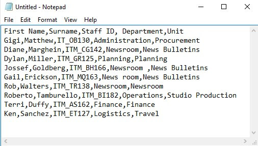
Getting data from a text file is common in Excel. A delimiter value separates each column. For example, look at the below data.

Step 1: We will use Power Query to import this data and transform it into a format that Excel loves working with.

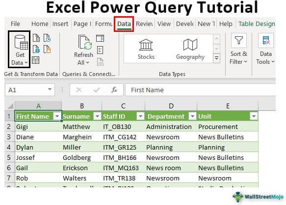
1. Go to the "Data" tab
2. Under "Get Data," click on "From File." 
3. Now, click on “From Text / CSV.”

Step 2: Now, Excel will ask you to choose the file you would like to import, so choose the file and click on “OK.”

It will display the data preview before it loads to the Power Query model. It looks like this.

As you can see above, it has automatically detected the delimiter as a “Comma” and segregated the data into multiple columns.

Step 3: Click “Load” at the bottom, which will load data to an Excel file in Excel table format.

Step 4: On the right side, we have a window called “Queries & Connections,” which suggests that data is imported through a Power Query.

Once the data is loaded to Excel, the connected text file should be intact Excel. So, go to the “Text File Data” and add two extra data lines.

Step 5: Now, come to Excel and select the table. It will show two more tabs: "Query” and “Table Design.”

Under “Query,” click on the “Refresh” button. It will refresh data with updated two new rows.

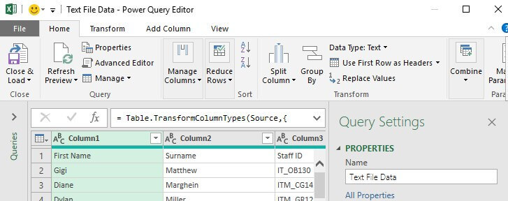
Step 6: There is another problem here, i.e., the first row is not captured as a column header.

Step 7: Click “Edit” under the “Query” tab to apply these changes.

Step 8: It will open the "Power Query Editor" tab.

Step 9: It is where we need a Power Query.

To make the first row a header, under the "Home" tab, click “Use First Row as Header.”

So, this will make the first row a column header. We can see this below.

Step 10: Click “Close & Load” under the "Home" tab. It will return data to Excel with modified changes.

The data looks in Excel like this. 

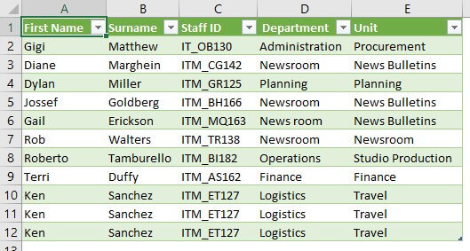
Without changing the actual position of the data, the Power Query modified the data.

You can study more on the subject like this Power Query tutorial using the Power Query in Excel article. 

Let us look at some of the frequently used tools in Power Query in this Power Query Tutorial:

1. Remove Rows: Right-click or use “Remove Rows” to delete top, bottom, or any required rows that are blank.
2. Rename Columns: To rename columns, you can double-click the column headers or use the Transform tab and choose Rename.
3. Filter Data: Select the columns you want to filter. Click the drop-down arrow next to the column header and use the filter icons in the header row.
4. Split Columns: You can split text by delimiter using Split Column in the ribbon.
5. Merging Queries: You can go to the Home tab and choose “Merge Queries." Then, select the queries you wish to merge and choose the matching columns. Specify what type of join you need and click OK. 

Use this to carry forward non-blank values in blank cells — very useful for nested data.

Unless you have a good knowledge of Power Query, it may be a little confusing when you look at the Power Query window.. So, here’s a brief introduction to the Power Query window.

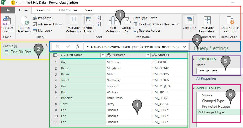
1. Query Editor Ribbon - This is just like the MS Excel ribbons. Under each ribbon, we have several features to work with.
2. List of Queries - This indicates all the tables imported to Excel in this workbook.
3. Formula Bar - It is similar to the formula bar in Excel, but here it is M Code.
4. Data Preview - It gives the preview of the data of the selected query table.
5. Properties - These are the properties of the selected table. You can name your query here.
6. Applied Steps - The most important part! All the applied steps in the Power Query are displayed here in chronological order. We can undo actions by deleting the queries. One can add, remove, reorder, or edit the steps if required.

This is an introductory tutorial to the Excel Power Query model. We have many other applications of Power Query a which we will see in the upcoming articles.

• The Power Query is an add-in for Excel 2010 and 2013, so we must install it manually.
• In Excel 2016, the Power Query is under the "Data" tab in the "Get & Transform Data" section.