Lookup Table In Excel

Last Updated :

21 Aug, 2024

Blog Author :

Edited by :

Reviewed by :

Table Of Contents

What Is LOOKUP Table In Excel?

LOOKUP table in Excel is a named table used with the VLOOKUP function to find any data. When we have a large amount of data and do not know where to look, we can select the table and name it. While using the VLOOKUP function, instead of providing the reference, we can type the table’s name as a reference to look up the value known as an Excel Lookup Table.

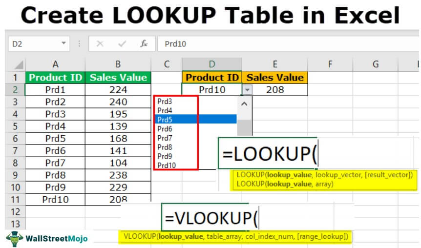
For example, we can use the LOOKUP() or the VLOOKUP() functions to look for the data in the table, as shown below.

What Is LOOKUP Table In Excel?

The LOOKUP Table in Excel helps users find the lookup_value using the LOOKUP function.
In Excel, VLOOKUP is the most commonly used LOOKUP function. Another important lookup function is HLOOKUP. Therefore, V stands for vertical lookup in VLOOKUP, and H stands for horizontal lookup in HLOOKUP.
The LOOKUP function helps us select the table from left to right, variable range by variable range, whereas in the VLOOKUP function, we can select the entire dataset, which also considers from left to right.
For the range_lookup arguments, if we are looking for the exact match, then FALSE or 0 is the input, and if we are looking for the approximate match, then TRUE or 1 is the input.

How To Create A Lookup Table In Excel?

We can fetch the available data and other information from different worksheets and workbooks using these LOOKUP functions, namely,

Create a Lookup Table Using VLOOKUP function.
Use LOOKUP Function to Create a Lookup Table in Excel.
Use INDEX + MATCH Function.

#1 - Create a Lookup Table using VLOOKUP Function

As we said, VLOOKUP is the traditional lookup function most users use regularly.

The syntax of the VLOOKUP function is,

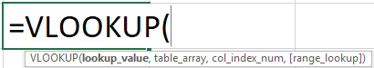
The arguments of the VLOOKUP function are,

lookup_value is the available value based on which we are trying to fetch the data from the other table.
table_array is the main table where all the information resides.
col_index_num is the column of the table_array from which we want the data. So, we must mention the column number here.
range_lookup helps choose whether we are looking for an exact or an approximate match.

Example of VLOOKUP Function:

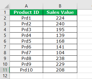
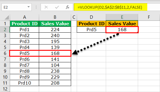
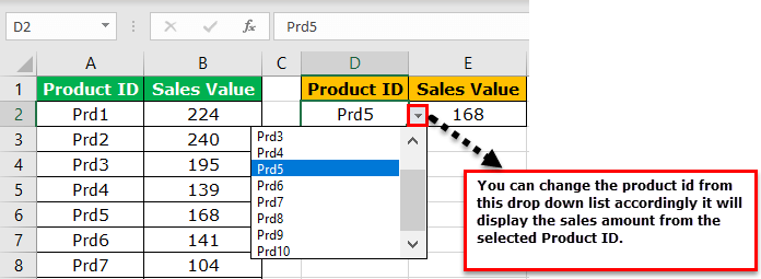
Assume below is the data you have of product sales and their sales amount.

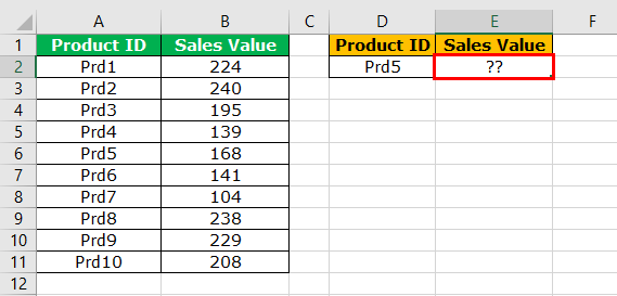
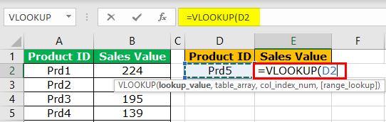
Now, in cell D2, we have one product ID, and using this product ID, we have to fetch the sales value using VLOOKUP.

The steps to use the VLOOKUP function are as follows:

We must apply the VLOOKUP function and open the formula first.
The first argument is the lookup_value. It is our base or available value. So, we must select cell D2 as the reference.
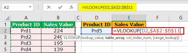
Next is the table_array. It is nothing but our main table where all the data resides. So, select the table_array as A2 to B11.
Now, press the F4 function key to make it an absolute excel reference. It will insert the dollar symbol into the selected cell.
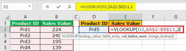
The next argument is the column index number from the selected table from which column we are looking for the data. In this case, we have chosen two columns, and we need the data from the second column, so we must mention 2 as the argument.
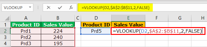
The final argument is range_lookup, i.e., type of lookup. Since we are looking at an exact match, we must select FALSE or insert zero as the argument.
Close the bracket and press the “Enter” key. We should have the sales value for the product ID Prd5.
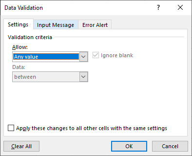
What if we want the sales data for the product if Prd6? Of course, we can enter directly, but this is not the right approach. Rather, we can create the drop-down list in excel allow the user to select from the drop-down list. Press ALT + A + V + V in cell D2. It is the shortcut key, which is the shortcut key to create data validation in excel.
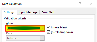
Select the “LIST” from the “Allow:” drop-down.
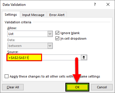
In the “SOURCE:” select the Product ID list from A2 to A11, and click “OK”.

Finally, we have the list of products in cell D2, as shown below.

#2 - Use LOOKUP Function to Create a LOOKUP Table in Excel

Instead of VLOOKUP, we can also use the LOOKUP function in excel as an alternative.

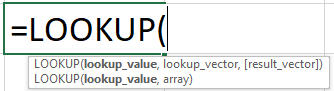
The syntax of the LOOKUP function is,

The arguments of the LOOKUP function are,

lookup_value is the base value or available value.
lookup_vector is nothing but a lookup_value column in the main table.
result_vector is nothing but requires a column in the main table.

Example of LOOKUP Function:

The steps to use the LOOKUP function are,

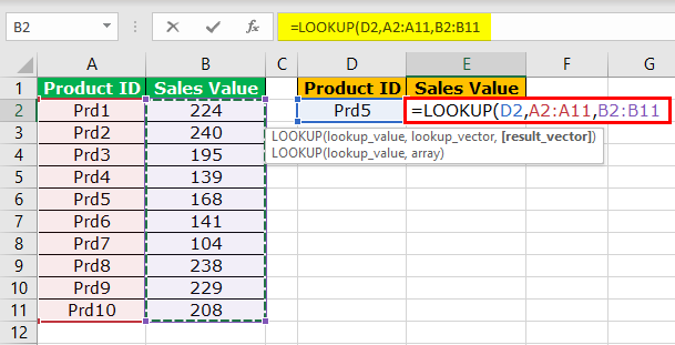
Step 1: We must open the LOOKUP function now.

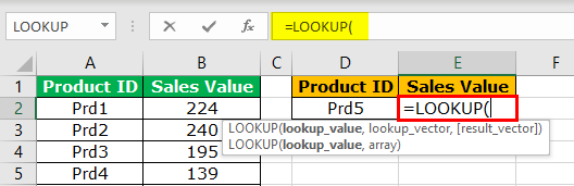
Step 2: The lookup_value is the product ID, so select the D2 cell.

Step 3: The lookup_vector is nothing but the product ID column in the main table. So, select A1 to A11 as the range.

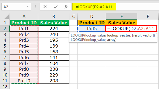
Step 4: Next is the results vector. It is nothing but from which column we need the data to be fetched. In this case, from B1 to B11, we want the data to be brought.

Step 5: Close the bracket, and press the “Enter” key to close the formula. We should have sales value for the selected product ID.

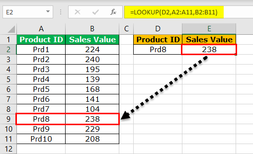
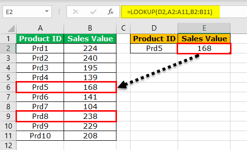
Step 6: Change the product ID to see a different result.

#3 - Use INDEX + MATCH Function

The VLOOKUP function can fetch the data from left to right, but with the help of the INDEX Function and MATCH formula in excel, we can bring data from anywhere to create a LOOKUP Excel table.

The steps to use the INDEX and the MATCH are,

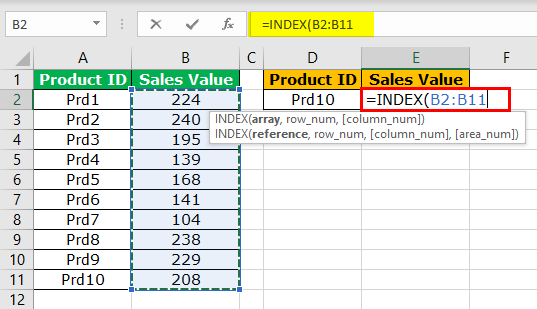
Step 1: Open the INDEX formula Excel first.

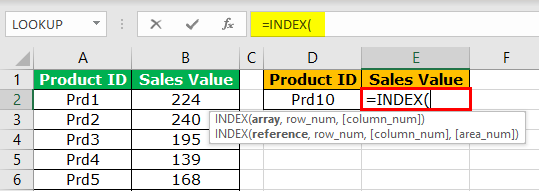
Use INDEX + MATCH Step 1 (lookup table in excel)

Step 2: Select the result column in the main table for the first argument.

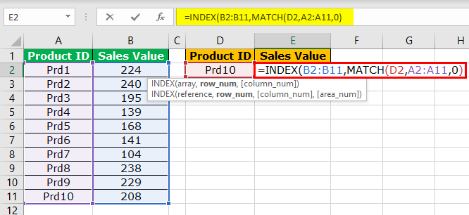
Use INDEX + MATCH Step 2 (lookup table in excel)

Step 3: To get the row number, we need to apply the MATCH function. Refer to the below image for the MATCH function.

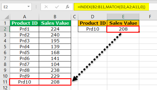
Use INDEX + MATCH Step 3 (lookup table in excel)

Step 4: Close the bracket and close the formula. We will have results, as shown below.

Important Things To Note

The LOOKUP should be the same as in the main table in Excel.
The VLOOKUP function works from left to right, not from right to left.
In the LOOKUP function, we need to select the result column and need not mention the column index number, unlike VLOOKUP.

Frequently Asked Questions (FAQs)

1. Where is the VLOOKUP function found in Excel?

The VLOOKUP function is found as follows:

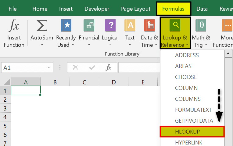
First, choose an empty cell → select the “Formulas” tab → go to the “Function Library” group → click the “Lookup & Reference” option drop-down → select the “VLOOKUP” function, as shown below.

LOOKUP Table in Excel - FAQ 1

Similarly, we can insert the LOOKUP function, as we can see the function available above the VLOOKUP function.

2. Where is the HLOOKUP function found in Excel?

The HLOOKUP function is found as follows:

First, choose an empty cell → select the “Formulas” tab → go to the “Function Library” group → click the “Lookup & Reference” option drop-down → select the “HLOOKUP” function, as shown below.

LOOKUP Table in Excel - FAQ 2

3. Why is the LOOKUP Table in Excel not working?

A few reasons the LOOKUP Table in Excel may not work are,

• The table_array is modified, and the Lookup table did not get updated automatically. In such scenarios, we can refresh the table to display the updated data.
• The dataset linked to the LOOKUP formulas is deleted. So, there is no data to look up or display.

Download Template

This article must help understand Lookup Table in Excel with its formulas and examples. You can download the template here to use it instantly.