AVERAGE Function in Excel

The AVERAGE function in Excel calculates the arithmetic mean of the supplied values. Such values can be numbers, percentages or times. In the mean (or average), the sum of all the items is divided by the number of items on the list. Apart from numbers, an average of Boolean values (true and false) can also be found if they are typed directly in the AVERAGE formula.

For example, the formula “=AVERAGE(10,24,35,true,false)” returns 14. The “true” and “false” values are counted as 1 and 0 respectively. So, the mean is (10+24+35+1+0)/5=14.

The purpose of using the AVERAGE function in Excel is to calculate the center or mean of a list. A mean includes every value of the list in the calculation. As a result, it is impacted by the extreme values or outliers (very small or very big values) of a list. The AVERAGE function is categorized as a Statistical function of Excel.

The syntax of the AVERAGE function of Excel is shown in the following image:

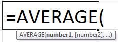
The AVERAGE function of Excel accepts the following arguments:

• Number 1: This is the first number for which the average is to be calculated.
• Number 2, number 3,…number n: These are the subsequent numbers for which the average is to be calculated.

The numbers can be supplied as direct numbers, named ranges or cell references containing numeric values. The first number is required, while the subsequent numbers are optional. However, for computing an average, at least two numbers are needed.

Note: The output of other Excel functions can also serve as an input to the AVERAGE function. However, such an output must necessarily be a numeric value.

The features of the AVERAGE function of Excel are listed as follows:

• It can be supplied with a maximum of 255 arguments in a single formula.
• It ignores the logical values (or Boolean values) if they have been supplied as cell references. However, logical values entered directly in the formula are counted by the function.
• It counts those cell references that contain numbers formatted as text.
• It treats the text strings as follows:
  • If the entire range reference consists of a few numbers and some text strings, the average of only the numbers is returned. In this case, the text strings supplied in the range reference are ignored by the function.
  • If the entire range reference consists of text strings, the “#DIV/0!” error is returned by the function.
  • If text strings are entered directly in the formula, it returns the “#VALUE!” error.
• It excludes the empty cells from the count. But, the cells containing the number zero are counted.
• It returns an error if the arguments supplied are error values.

Note: To include the zero values and exclude the empty cells from the count, follow the listed steps:

1. Click “options” from the File tab. The “Excel options” window opens.
2. Click “advanced” displayed on the left side.
3. Under “display options for this worksheet,” select the checkbox of “show a zero in cells that have zero value.”

The zero values of cells will be displayed and included in the count by the AVERAGE function of Excel. Deselecting the checkbox in point “c” will hide the zero values and display empty cells in their place.

The AVERAGE function is one of the most used functions of Excel. It is frequently used in the financial sector to calculate the average revenue generated by an organization in a specific time period. It is also used to do financial modeling and analyze datasets.

Let us consider a few examples to understand the working of the AVERAGE function of Excel.

Example #1–Average in Five Different Cases

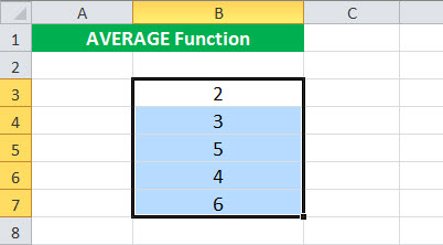
The following image shows a list of numbers in the range B3:B7. Use the AVERAGE function of Excel to perform the tasks stated within the following cases:

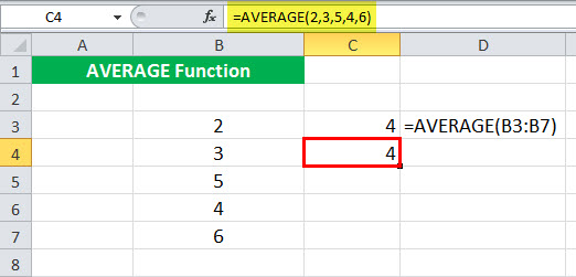
• Case 1: Calculate the average by supplying a vertical range reference.
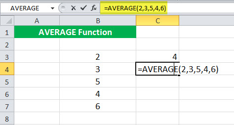
• Case 2: Calculate the average by supplying the numbers directly to the function.
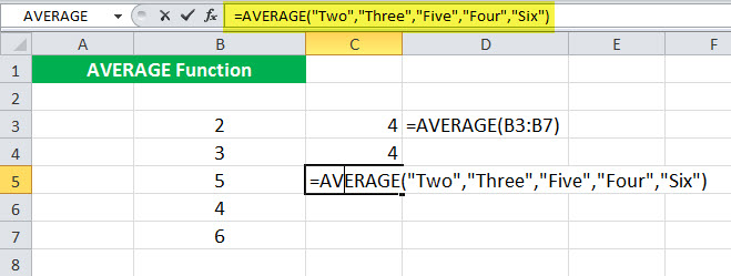
• Case 3: Calculate the average by supplying the numbers in words. Enclose the text strings within double quotation marks.
• Case 4: Calculate the average by supplying the references of cells containing the number names.
• Case 5: Calculate the average by supplying the numbers directly within double quotation marks.

Write a conclusion for each case.

Case 1: Supply a vertical range reference

The steps are listed as follows:

Step 1: Enter the following formula in cell C3.

“=AVERAGE(B3:B7)”

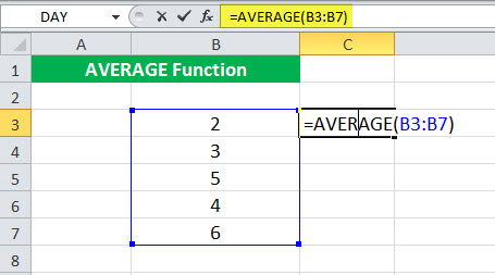
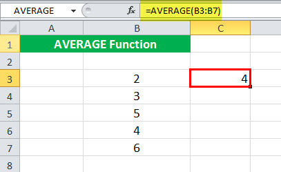
Step 2: Press the “Enter” key. The output in cell C3 is 4. So, the mean of the given numbers is 4. This is shown within a red box in the following image.

Conclusion: For calculating the average, the numbers can be supplied as a range reference. It is also possible to supply cell references of non-adjacent cells.

Simply select the cell or range in order to supply it to the AVERAGE function. Further, ensure that the non-contiguous cells or ranges are separated by commas.

Case 2: Supply the numbers directly to the AVERAGE function

The steps are listed as follows:

Step 1: Enter the following formula in cell C4.

“=AVERAGE(2,3,5,4,6)”

Step 2: Press the “Enter” key. The output is shown in cell C4 of the following image. Hence, the mean is again 4.

Conclusion: It is possible to supply the numbers directly to the AVERAGE function. One need not enclose such numbers within double quotation marks.

However, when there are too many numbers in the list, it becomes difficult to enter them directly. In such cases, it is easier to supply cell references.

Case 3: Supply the numbers in words

The steps are listed as follows:

Step 1: Enter the following formula in cell C5.

“=AVERAGE("Two","Three","Five","Four","Six")”

Step 2: Press the “Enter” key. The output in cell C5 is the “#VALUE!” error. This is shown in the following image.

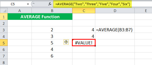
Conclusion: When the number names are supplied directly to the AVERAGE function, it returns the“#VALUE!” error. This implies that the AVERAGE function does not work with text strings, even if such strings are enclosed within double quotation marks.

Case 4: Supply the references to cells containing the number names

The steps are listed as follows:

Step 1: Write the names of the numbers in the range A3:A7. Next, enter the following formula in cell C6.

“=AVERAGE(A3:A7)”

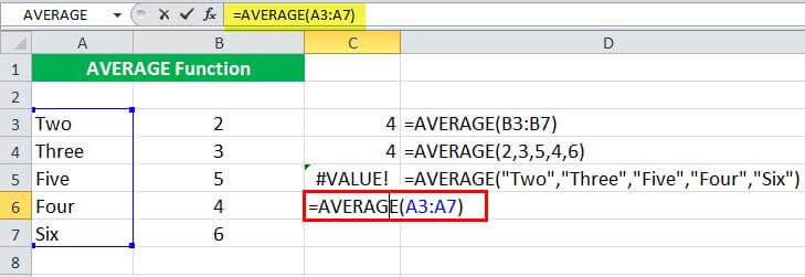
Step 2: Press the “Enter” key. The output in cell C6 is the “#DIV/0!” error. This is shown in the following image.

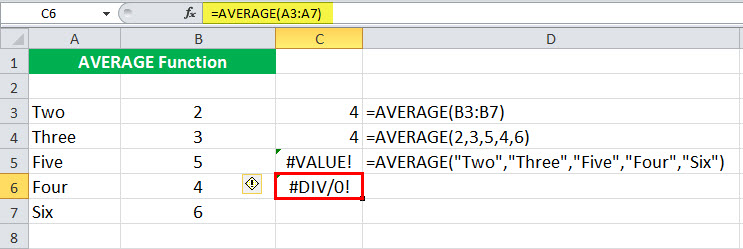
Conclusion: If number names are supplied as cell references, the AVERAGE function returns the “#DIV/0!” error. This implies that whether text strings are supplied directly or as cell references, the AVERAGE function does not work with them.

Notice the green triangles appearing on the top-left corner of cells C5 and C6. These triangles indicate that there is an error in the formulas of these cells.

Note: To include the text strings supplied as cell references, use the AVERAGEA function of Excel. This function counts such text strings as zero and ignores the empty cells. However, the text strings entered directly in the AVERAGEA formula can cause errors.

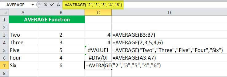
Case 5: Supply the numbers directly within double quotation marks

The steps are listed as follows:

Step 1: Enter the following formula in cell C7.

“=AVERAGE(“2”,“3”,“5”,“4”,“6”)”

Step 2: Press the “Enter” key. The output in cell C7 is 4. Hence, the mean is 4. This is shown within a red box in the following image.

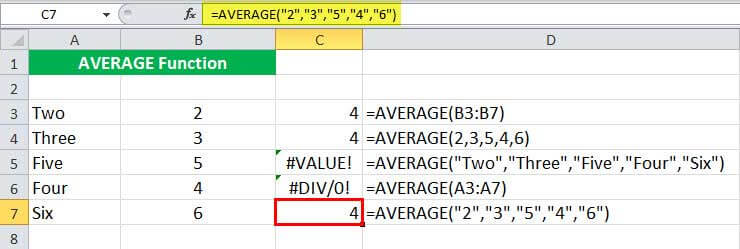
Conclusion: If numbers are supplied directly within double quotation marks, the AVERAGE function returns their average (or mean). Hence, whether numbers are supplied as cell references or direct values (with or without double quotation marks), the AVERAGE function returns their mean.

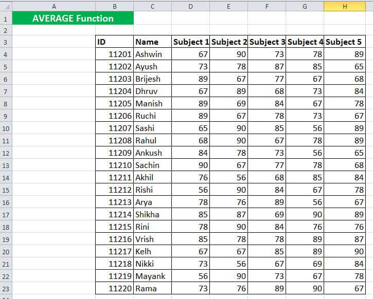
Example #2–Average by Supplying a Horizontal Range Reference

The following image shows the names (column C), IDs (column B), and scores (in five subjects in columns D to H) of 20 students of a class. Given that the maximum marks of each subject are 100, calculate the average score obtained by each student.

Use the AVERAGE function of Excel.

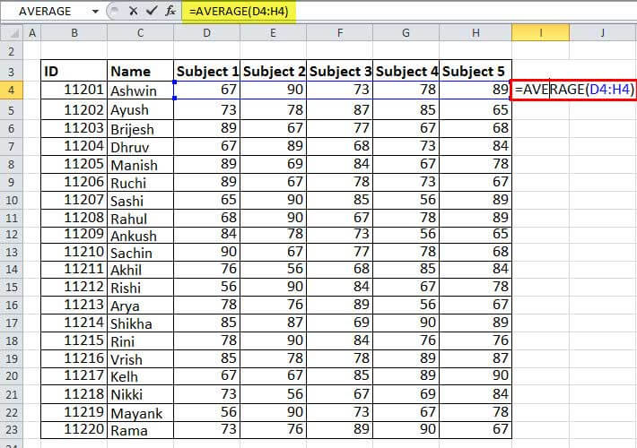
The steps to calculate the average are listed as follows:

Step 1: Enter the following formula in cell I4.

“=AVERAGE(D4:H4)”

So, we have supplied the cell references of row 4 to the AVERAGE function of Excel.

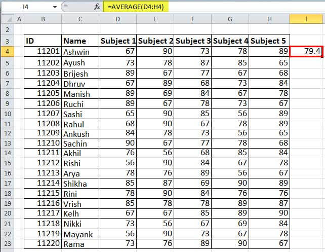
Step 2: Press the “Enter” key. The output in cell I4 is 79.4. Hence, the average score of the student Ashwin is 79.4.

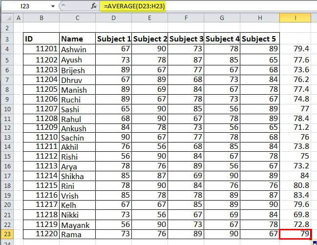
Step 3: Drag the formula of cell I4 till cell I23. For dragging, use the excel fill handle appearing at the bottom-right side of cell I4.

The outputs are shown in the following image. The formula bar shows the formula of the currently selected cell (I23).

Example #3–Average and Maximum Average Revenue by AVERAGE, LOOKUP, and MAX Functions

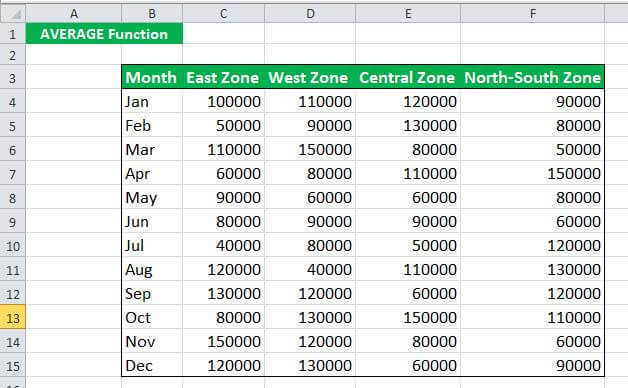
The following image shows the monthly revenues (in $ in columns C to F) generated by an organization from four zones, namely, east, west, central, and north-south. We want to perform the listed tasks:

1. Calculate the average revenue for each month.
2. Calculate the average revenue for each zone.
3. Find the zone with the maximum average revenue.

Use the AVERAGE function of Excel for tasks “a” and “b.” For task “c,” use the LOOKUP and MAX functions. Further, explain the formula used for task “c.”

a. The steps to calculate the average revenue for each month are listed as follows:

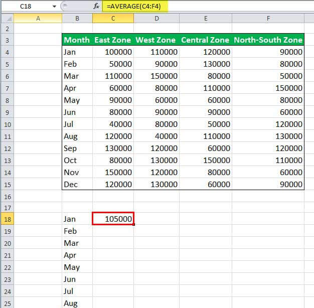
Step 1: Enter the following formula in cell C18.

“=AVERAGE(C4:F4)”

Since the average for each row of the dataset needs to be calculated, we have supplied the range reference of row 4.

Step 2: Press the “Enter” key to obtain the output. This is shown in cell C18 of the following image. So, the average revenue for January is $105,000.

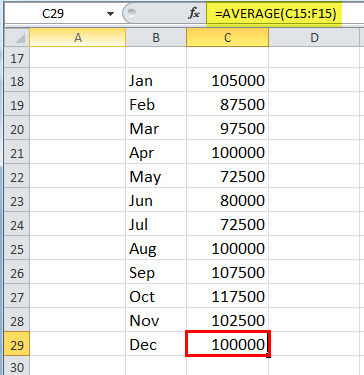
Step 3: Drag the formula of cell C18 till cell C29 with the help of the fill handle. The average revenues for all the months are shown in the following image. In this image, the formula bar displays the formula of the currently active cell (C29).

b. The steps to calculate the average revenue for each zone are listed as follows:

Step 1: Enter the following formula in cell G18.

“=AVERAGE(C4:C15)”

This time we supply the cell references of column C in the AVERAGE formula. This is because the average for the entire column needs to be calculated.

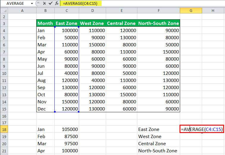
Step 2: Press the “Enter” key. The output of cell G18 is shown in the following image. Likewise, we have entered the following formulas in cells G19, G20, and G21 respectively:

• “=AVERAGE(D4:D15)”
• “=AVERAGE(E4:E15)”
• “=AVERAGE(F4:F15)”

Hence, the averages for each zone have been calculated in the range G18:G21.

c. The steps to find the zone with the maximum average revenue are listed as follows:

Step 1: Enter the following formula in cell H18.

“=LOOKUP(MAX(G18:G21),G18:G21,F18:F21)”

This is shown in the following image.

Step 2: Press the “Enter” key. The output is shown in the following image. Hence, the average revenue of the west zone is maximum.

Explanation of the formula: In the formula of step 1, we have used the vector form of the LOOKUP function. This formula works as follows:

1. The MAX function looks for the maximum number of the range G18:G21. The output of the MAX function is 100000. This output becomes the “lookup_value” of the LOOKUP function.
2. Next, the LOOKUP function searches the number 100000 (lookup_value) in the range G18:G21 (lookup_vector). It returns the result from the range F18:F21 (result_vector). So, the given “lookup_value” corresponds with the west zone.

Hence, the output of the formula of step 1 is “west zone.”

Note: The LOOKUP function searches for a value (lookup_value) in a one-row or one-column range (lookup_vector) and returns a corresponding match from the same position of another range (result_vector). The MAX function returns the maximum number from a dataset of numeric values.

For the syntax of the LOOKUP and MAX functions, click the hyperlinks of points “b” and “a” respectively.

Example #4–Average of Top Four Scores by AVERAGE and LARGE Functions

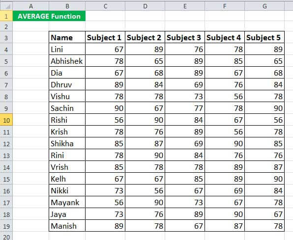
The following image shows the names (column B) and scores (columns C to G) of 16 students in five subjects. We want to perform the listed tasks:

1. Calculate the average of five scores of the student Lini (row 4). Use the AVERAGE function of Excel.
2. Calculate the average of the top four scores of each student. Use the AVERAGE and LARGE functions of Excel.

Explain the formula used for task “b.”

a. The steps to calculate the average of the five scores of row 4 are listed as follows:

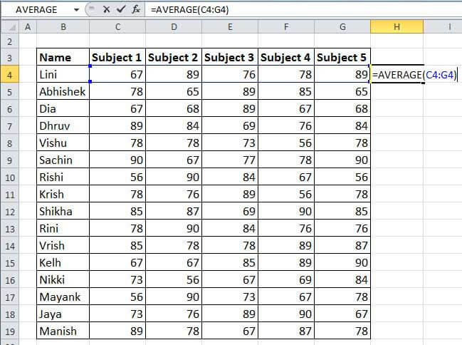
Step 1: Enter the following formula in cell H4.

“=AVERAGE(C4:G4)”

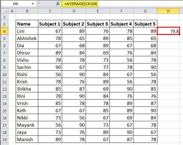
Step 2: Press the “Enter” key. The output is 79.8, as shown in the following image. Hence, Lini’s average of five scores is 79.8.

Note: To find the average (of five scores) for all the students, simply drag the formula of cell H4 till cell H19. For dragging, use the fill handle at the bottom-right corner of cell H4.

b. The steps to calculate the average of the top four scores of each student are listed as follows:

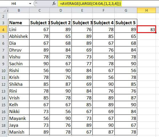
Step 1: Enter the following formula in cell H4.

“=AVERAGE(LARGE(C4:G4,{1,2,3,4}))”

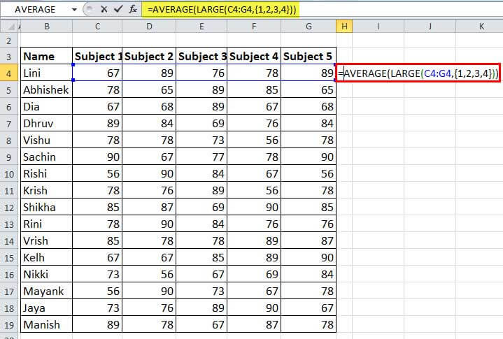
Step 2: Press the “Enter” key. The output is shown in cell H4 of the following image. Hence, Lini’s average of the top four scores is 83.

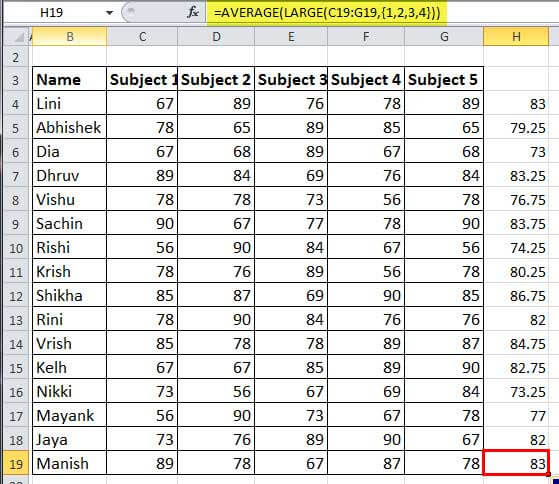
Step 3: Drag the formula of cell H4 till cell H19. The outputs for all rows are shown in the following image. Notice that all these outputs are the averages of the top four scores of each student.

Explanation of the formula: In the formula of step 1, the inner function (LARGE function) is processed first, followed by the outer function (AVERAGE function). This formula works as follows:

1. An array of numbers {1,2,3,4} has been supplied to the LARGE function. These numbers represent the position from which values will be returned. So, the LARGE function searches for the first highest, second highest, third highest, and fourth highest values in the range C4:G4. As a result, the LARGE function returns an array of numbers, which is {89,89,78,76}.
2. The array of numbers returned by the LARGE function {89,89,78,76} serves as the argument of the AVERAGE function. The AVERAGE function calculates the average of these numbers, which is (89+89+78+76)/4=83.

Likewise, the average of the top four scores has been obtained for all the students of the range B4:B19.

Note: The LARGE function returns a value from the specified position of the supplied range. This position begins from the highest value of the dataset. So, the number 1 corresponds to the maximum value of the dataset, 2 corresponds to the second highest value, 3 corresponds to the third highest value, and so on.

For the syntax of the LARGE function, click the hyperlink given in point “a” of the preceding explanation.

Example #5–Average of Last Three Numbers by AVERAGE, LOOKUP, LARGE, IF, ISNUMBER, and ROW Functions

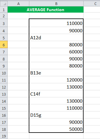
The following image shows some numeric and textual values in column B. Calculate the average of the last three numeric values, which are in cells B15, B17, and B18.

Use the AVERAGE, LOOKUP, LARGE, IF, ISNUMBER, and ROW functions of Excel. Further, explain the formula used for the given task.

The steps to calculate the average of the last three numeric cells are stated as follows:

Step 1: Enter the following formula in cell C3.

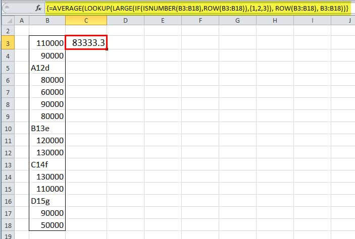
“=AVERAGE(LOOKUP(LARGE(IF(ISNUMBER(B3:B18),ROW(B3:B18)),{1,2,3}),ROW(B3:B18),B3:B18))”

Step 2: Press the keys “Ctrl+Shift+Enter” together. For Excel for Mac, press the keys “Command+Shift+Enter.”

Once the CSE (Ctrl+Shift+Enter) keys are pressed, the formula is enclosed within curly braces. This is shown in the following image. The output is also shown in cell C3.

Hence, the average of the last three numeric values (110000, 90000, and 50000) is 83333.3.

Explanation of the formula: The formula of step 1 works as follows:

a. In the formula “ISNUMBER(B3:B18),ROW(B3:B18),” the ROW function returns the row numbers of the range B3:B18. So, the ROW function returns the following array of values:

{3;4;5;6;7;8;9;10;11;12;13;14;15;16;17;18}.

b. The ISNUMBER function processes each value returned by the ROW function. The ISNUMBER function returns “true” if a cell of column B contains a number. It returns “false” if a cell of column B contains a text string. Consequently, the ISNUMBER function returns the following array of logical values:

{TRUE;TRUE;FALSE;TRUE;TRUE;TRUE;TRUE;FALSE;TRUE;TRUE;FALSE;TRUE;TRUE;FALSE;TRUE;TRUE}

c. Next, the IF function operates. The “logical_test” of the IF function is “ISNUMBER(B3:B18)” and the “value_if_true” is “ROW(B3:B18).” The “value_if_false” has been omitted. Therefore, the IF function processes each value of the array returned by the ISNUMBER function. The IF function returns the row number for each “true” value and “false” for each “false” value. So, the IF function returns the following array of values:

{3;4;FALSE;6;7;8;9;FALSE;11;12;FALSE;14;15;FALSE;17;18}

d. The LARGE function has been supplied the array {1,2,3} in the formula “LARGE(IF(ISNUMBER(B3:B18),ROW(B3:B18)),{1,2,3}).” So, the LARGE function searches for the first highest, second highest, and third highest values in the array returned by the IF function. The LARGE function returns the following array of three values:

{18,17,15}

e. Next, the LOOKUP function processes the formula “LOOKUP({18,17,15},ROW(B3:B18),B3:B18).” So, the LOOKUP function searches for the values 18, 17, and 15 in the array returned by the formula “ROW(B3:B18).” The array returned by this ROW formula is the same as that of point “a.” Therefore, the LOOKUP function returns a corresponding match of the values 18, 17, and 15 from the range B3:B18. As a result, the following array is returned by the LOOKUP function:

{50000,90000,110000}

f. Finally, the AVERAGE function calculates the mean of the three values returned by the LOOKUP function. It returns 83333.3 as the average.

Notice that the formula of step 1 works as an array formula as it has been completed by pressing the CSE (Ctrl+Shift+Enter) keys. Therefore, the LOOKUP function also returns an array of corresponding matches (50000, 90000, and 110000) for the multiple “lookup_values” (18, 17, and 15) supplied to it.

However, the regular LOOKUP function looks for a single “lookup_value” and returns a single corresponding match. Moreover, it is completed by pressing the “Enter” key.

Note 1: The ROW function returns the row numbers of the supplied cell reference. The ISNUMBER function checks whether the supplied value or cell reference is numeric or not. It returns “true” if the supplied value (or reference) is numeric, otherwise it returns “false.”

The IF function checks whether the supplied condition (logical_test) is true or false. If the condition is true, it returns the “value_if_true.” If the condition is false, it returns the “value_if_false.” If the logical test evaluates to false and the “value_if_false” is omitted, the IF function returns “false.”

For the syntax of the ROW, ISNUMBER, and IF functions, click the hyperlinks given in points “a,” “b,” and “c” of the preceding explanation. The definitions of the LOOKUP and LARGE functions are given in the notes at the end of examples #3 and #4 respectively.

Note 2: To view the array returned by each function, follow the listed steps:

1. Select cell C3 that contains the formula.
2. Double-click within the selected cell. Alternatively, press the key F2 to enter the Edit mode.
3. Select that part of the formula whose array needs to be viewed. For instance, to view the array returned by the ISNUMBER function, select “ISNUMBER(B3:B18).”
4. Press the key F9 once a selection has been made in the preceding step.

To stop editing the formula, press the escape (Esc) key.

This has been a guide to the AVERAGE function in Excel. Here we explain how to calculate Average using AVERAGE formula in Excel along with examples and downloadable Excel templates. You may also look at these useful functions of Excel–

• Weighted Average Excel
• LARGE Function in Excel
• Weighted Average Formula
• SUMPRODUCT Function in Excel