What Is Excel Bar Chart?
Bar charts in Excel are one of the options found in the Charts group used to display the values in the bar-chart format. They represent the values in horizontal bars. Categories are displayed on the Y-axis in these charts, and values are shown on the X-axis.
To create or make a bar chart, a user needs at least two variables, i.e., independent and dependent variables.
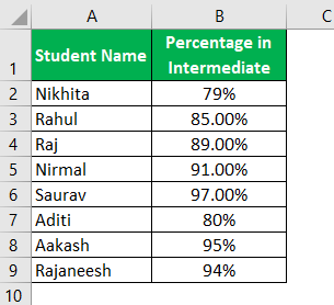
For example, consider the below table showing the marks obtained by students. Now, let us learn how to create bar chart in excel for the given data.

The steps used to create bar chart in excel are:
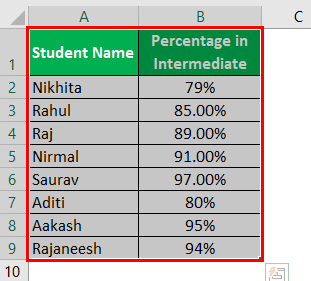
- Step 1: First, select the values in the table.
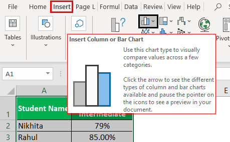
- Step 2: Next, go to Insert and click on Insert column or bar chart from the Charts group.
- Step 3: Choose the desired bar chart type.
As soon as we click on the chart type, Excel will display the values in the bar-chart type as shown in the image below.

Likewise, we can create bar chart in excel.
Key Takeaways
- Bar Chart in excel is used to display the values in bar chart format.
- A bar chart is only useful for small sets of data.
- The bar chart ignores the data if it contains non-numerical values.
- It is hard to use the bar charts if data is not arranged properly in the Excel sheet.
- Bar charts and column charts have a lot of similarities except for the visual representation of the bars in horizontal and vertical format. These can be interchanged with each other.
Explanation And Usage
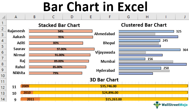
Before using bar chart in excel, let us learn the three types of bar charts in Excel.
- Stacked Bar Chart: It is also referred the segmented chart. It represents all the dependent variables by stacking them together and on top of other variables.
- Clustered Bar Chart: This chart groups all the dependent variables to display in a graph format. A clustered chart with two dependent variables is the double graph.
- 3D Bar Chart: This chart represents all the dependent variables in 3D representation.
How To Create A Bar Chart In Excel?
Creating bar chart in excel is easy. Let us see the steps used to create bar chart in excel;
- Step 1: Select the table.
- Step 2: Go to the Insert tab.
- Step 3: Click the drop-down button of the Insert Column or Bar Chart option from the Charts group.
- Step 4: Select the type of chart from the drop-down list.
Likewise, we can create bar chart in excel.
Examples
Example #1 – Stacked Bar Chart
This example illustrates how to create a stacked bar graph in simple steps.
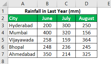
First, we must enter the data into the Excel sheets in the table format, as shown in the figure.

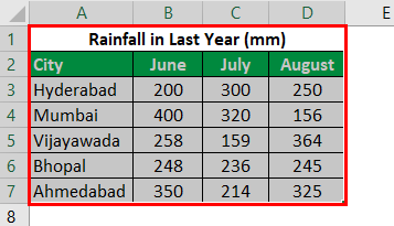
Then, select the entire table by clicking and dragging or placing the cursor anywhere in the table, and then, press CTRL+A to select the whole table.

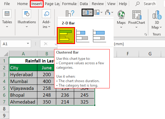
Next, we will go to the Insert tab and move the cursor to the insert bar chart option.

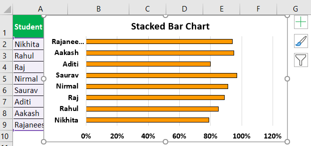
Under the 2D bar chart, we select the stacked bar chart, as shown in the figure below.

We may see the stacked bar chart as shown below.

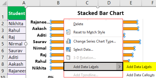
We will add Data Labels to the data series in the plotted area.
We will click on the chart area to select the data series.

Now, as shown in the screenshot, we will right-click on the data series and choose the add data labels to add the data label option.

We can move the bar chart to the desired place in the worksheet. Then, we can click on the edge and drag it with the mouse.

We can change the design of the bar chart utilizing the various options available, including changing color, changing the chart type, and moving the chart from one sheet to another sheet.

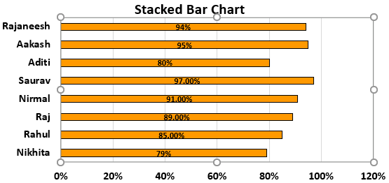
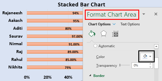
We get the following stacked bar chart.
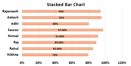
We can use the Format Chart Area to change color, transparency, dash type, cap type, and join type.


Example #2 – Clustered Bar Chart
This example illustrates how to create a clustered bar chart in simple steps.
- Step 1: As shown in the figure, we must enter the data into the Excel sheets in the Excel table format, as shown in the figure.
- Step 2: We must select the entire table by clicking and dragging or placing the cursor anywhere and pressing CTRL+A to choose the whole table.
- Step 3: We will go to the Insert tab and move the cursor to the insert bar chart option. Then, under the 2D Bar Chart, select the clustered bar chart shown in the figure below.
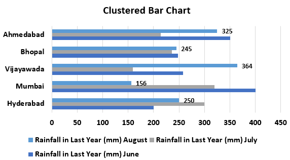
- Step 4: Next, we will add a suitable title to the chart, as shown in the figure.

- Step 5: Now, we will right-click on the data series and choose the add data labels to add the data label option, as shown in the screenshot.
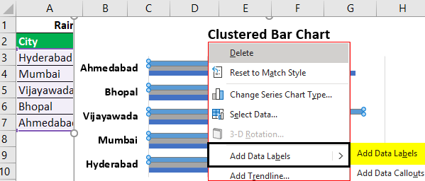
The data is added to the plotted chart, as shown in the figure.
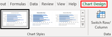
- Step 6: We will now apply to format to change the charts’ design using the chart’s Design and Format tabs, as shown in the figure.
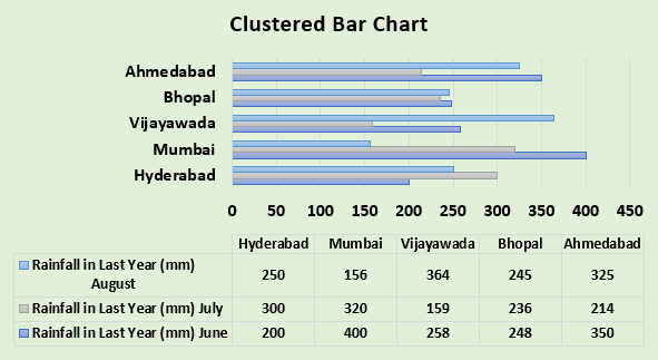
As a result, we can get the following chart.
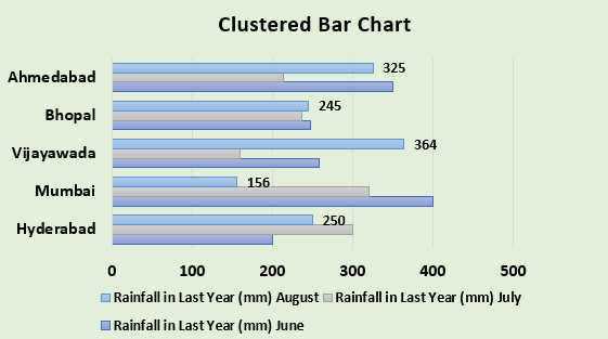
We can also change the chart’s layout using the Quick Layout feature.
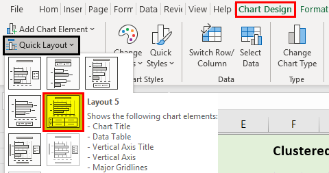
Therefore, we will get the following clustered bar chart.
Example #3 – 3D Bar Chart
This example illustrates creating a 3D bar chart in Excel in simple steps.
- Step 1: First, we must enter the data into the Excel sheets in the table format, as shown in the figure.
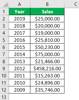
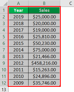
- Step 2: We will now select the whole table by clicking and dragging or placing the cursor anywhere and pressing CTRL+A to choose the table completely.
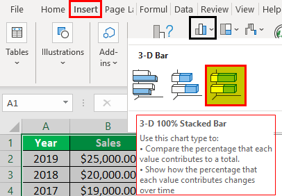
- Step 3: Next, we will go to the Insert tab and move the cursor to the insert bar chart option. Under the 3D Bar Chart, select the 100% stacked bar chart, as shown in the figure below.
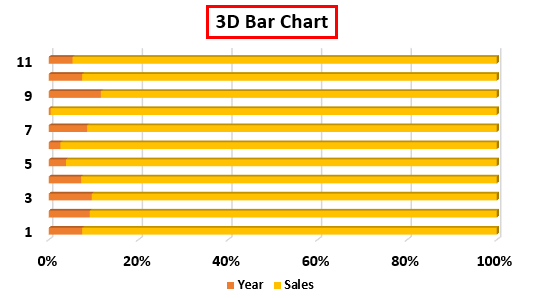
- Step 4: Now will add a suitable title to the chart, as shown in the figure.
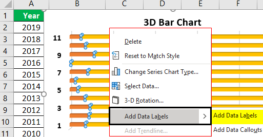
- Step 5: We will now right-click on the data series and choose Add Data Labels to add the data label option, as shown in the screenshot.
The data is added to the plotted chart, as shown in the figure.

Using the format chart area, we will apply the required formatting and design. As a result, we will get the following 3D bar chart.

Uses Of Bar Chart
Let us understand the uses of bar chart in Excel;
- Easier planning and making decisions based on the data analyzed.
- Determination of business decline or growth in a short time from the past data.
- Visual representation of the data and improved abilities in the communication of complex data.
- Comparing the different categories of data to enhance the proper understanding.
- Finally, summarize the data in the graphical format produced in the tables.
Important Things To Note
- We can turn any Excel data into a stacked bar graph that can display comparisons between categories of data, ranking, part-to-whole, deviation, or distribution.
- Bar Charts in excel compare parts of a whole with the ability to break down.
- We can also use the clustered bar chart to represent more than one data series in clustered horizontal columns when the data is complex and difficult to understand.
- In addition, we can also use a 3D bar chart to provide the chart’s title and define labels and values to make the chart more understandable.
Frequently Asked Questions (FAQs)
What is bar chart in excel?
Bar chart in excel is used to display small data into bar charts. There are bar charts, clustered bar charts, and 3D bar charts in excel.
What are independent and dependent variables?
- Independent Variable: This does not change concerning any other variable.
- Dependent Variable: This change concerns the independent variable.
How to create 2D bar chart in excel?
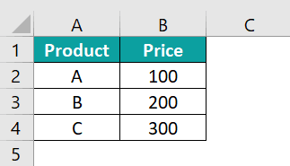
For example, consider the below table showing the price of various items. Now, let us learn how to create bar chart in excel.
The steps used to create bar chart in excel are:
• Step 1: First, select the values in the table.
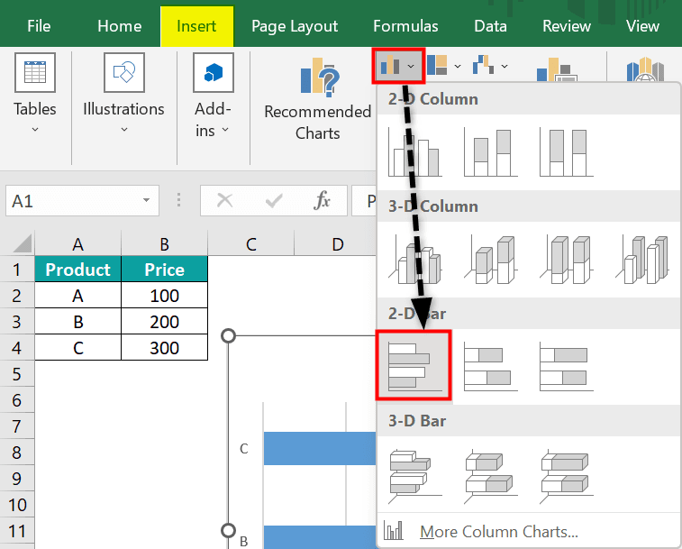
• Step 2: Next, go to Insert and click on Insert column or bar chart from the Charts group.
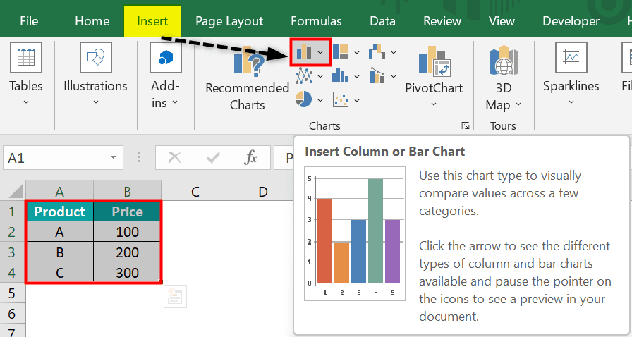
• Step 3: Choose the desired bar chart type. In our example, we have selected 2D clustered bar.
As soon as we click on the chart type, Excel will display the values in the bar-chart type as shown in the image below.
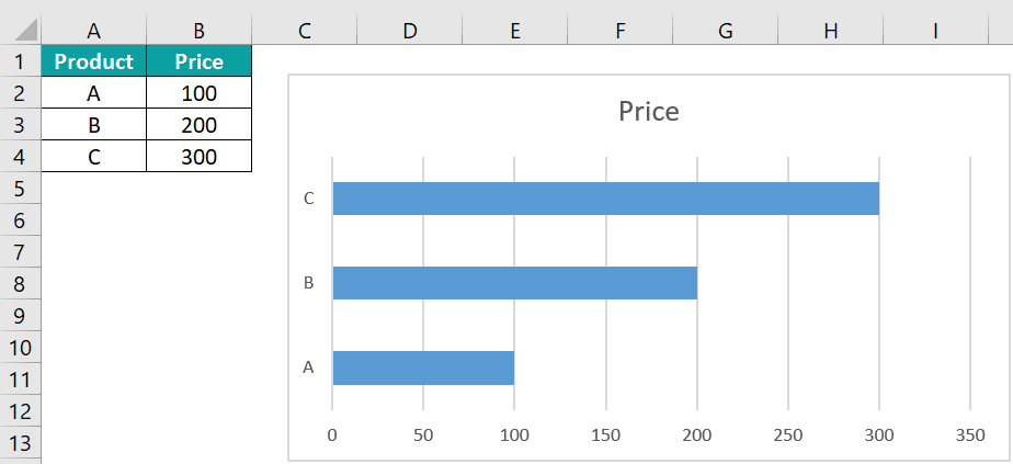
Likewise, we can create bar chart in excel.
Recommended Articles
This article is a guide to Bar Chart in Excel. We discuss how to create different types of bar chart in Excel (stacked, clustered, and 3D), along with examples. You can have a look at other articles on Excel functions: –