Sensitivity Analysis in Excel

Let us take the Finance example (Dividend discount model) below to understand this in detail.

Constant growth DDM gives us the Fair value of a stock as a present value of an infinite stream of dividends growing at a constant rate.

Gordon Growth formula is as per below –

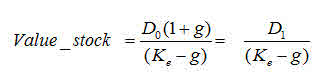
Where:

• D1 = Value of dividend to be received next year
• D0 = Value of dividend received this year
• g   = Growth rate of dividend
• Ke = Discount rate

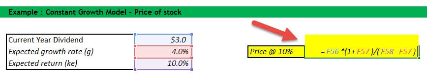
Now, let’s assume that we want to understand how sensitive the stock price is concerning the Expected Return (ke). There are two ways of doing this –

• Donkey way :-)
• What if Analysis

#1 – Donkey Way

Sensitivity Analysis in Excel using Donkey’s way is very straightforward but hard to implement when many variables are involved.

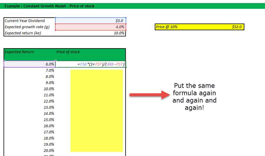
Do you want to continue making this given 1000 assumptions? Not!

Learn the following sensitivity analysis in excel technique to save yourselves from trouble.

#2 – Using One Variable Data Table

The best way to do sensitivity in excel is to use Data Tables. Data tables provide a shortcut for calculating multiple versions in one operation and a way to view and compare the results of all variations on your worksheet.

Below are the steps that you can follow to implement a one-dimensional sensitivity analysis in excel.

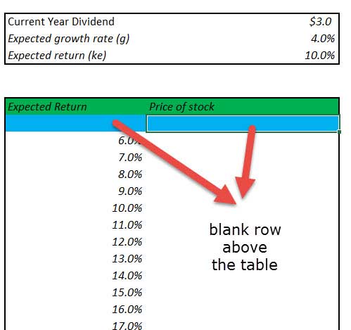
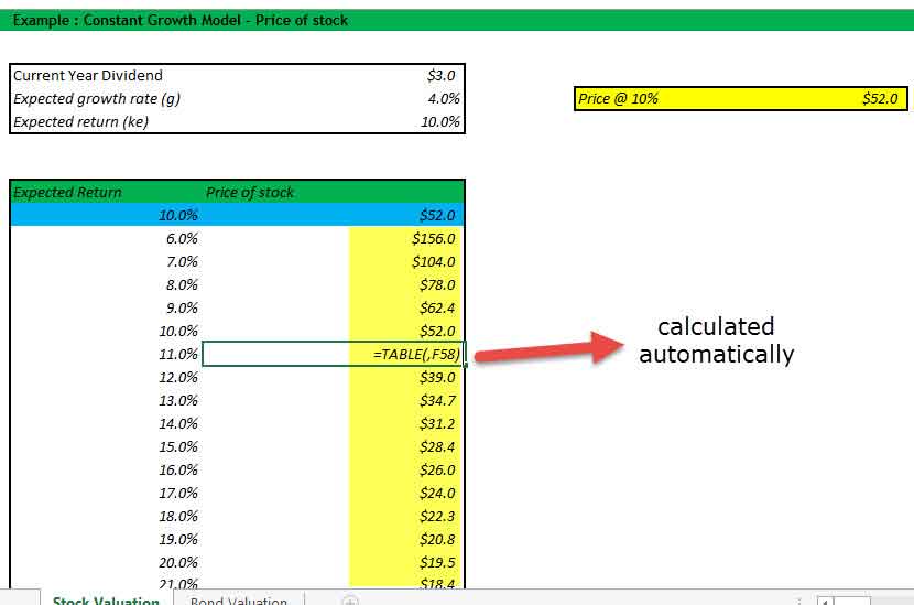
1. Create the table in a standard format.

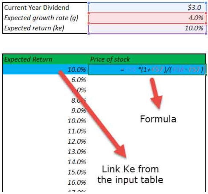
In the first column, you have the input assumptions. In our example, inputs are the expected rate of return (ke). Also, please note a blank row (colored in blue in this exercise) below the table heading. This blank row serves an important purpose for this one-dimensional data table, which you will see in Step 2.

2. Link the reference Input and Output as given the snapshot below.

The space provided by the blank row is now used to provide input (expected return Ke) and the output formula. Why is it done like this? We will use What if Analysis; this is a way to instruct Excel that for the Input (ke), the corresponding formula provided on the right-hand side should be used to recalculate all the other input.

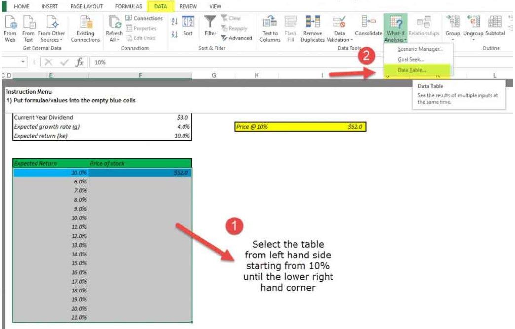
3. Select the What-if Analysis tool to perform Sensitivity Analysis in Excel.

It is important to note that this is sub-divided into two steps.
1. Select the table range starting from the left-hand side, starting from 10% until the lower right-hand corner of the table.
2. Click Data – What if Analysis – Data Tables

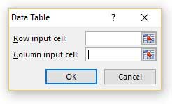
4. Data Table Dialog Box Opens Up.

The dialog box seeks two inputs – Row Input and Column Input. Since there is only one input ,Ke, is under consideration, we will provide a single column input.

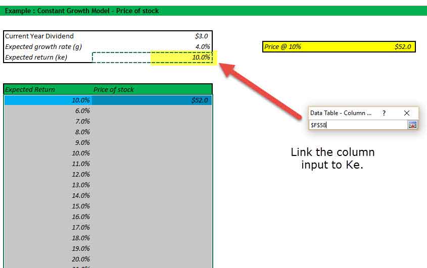
5. Link the Column Input

In our case, all input is provided in a column, and hence, we will link to the column input. Column input is linked to the Expected return (Ke). Please note that the input should be linked from the source and Not from the one inside the table..

6. Enjoy the Output

Data tables are very useful for Sensitivity analysis in excel, especially in the case of DCF. Once a base case is established, DCF analysis should always be tested under various sensitivity scenarios. Testing involves examining the cumulative effect of changes in assumptions (cost of capital, terminal growth rates, lower revenue growth, higher capital requirements, etc.) on the fair value of the stock.

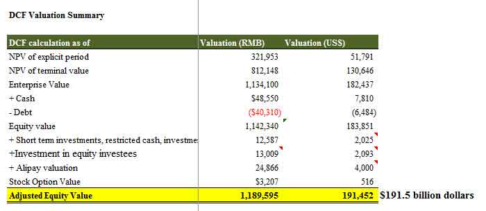
Let us take the sensitivity analysis in excel with a finance example of Alibaba Discounted Cash Flow Analysis.

With the base assumptions of the Cost of Capital as 9% and constant growth rate of 3%, we arrived at the fair valuation of $191.45 billion.

Let us assume that you do not fully agree with the Cost of Capital Assumptions or the growth rate assumptions I have taken in Alibaba IPO Valuation. You may want to change the assumptions and assess the impact on valuations.

One way is to change the assumptions and check each change’s results manually. (codeword – Donkey method!)

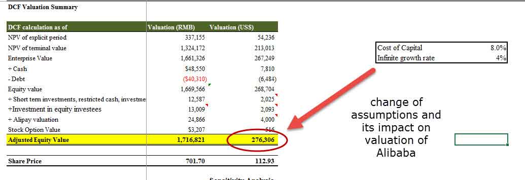
However, we are here to discuss a much better and more efficient way to calculate valuation using sensitivity analysis in excel that saves time and provides us with a way to visualize all the output details in an effective format.

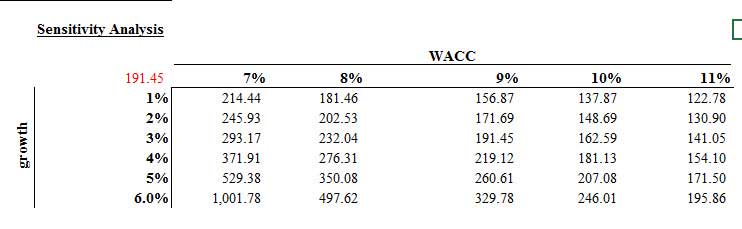
If we perform the What-if analysis in excel professionally on the above data, then we get the following output.

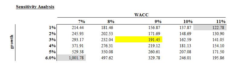
• Here, row inputs consist of changes in Cost of capital or WACC (7% to 11%)
• Column inputs consist of changes in growth rates (1% to 6%)
• The point of intersection is Alibaba Valuation. E.g. using our base case of 9% WACC and 3% growth rates, we get the valuation as $191.45 billion.

With this background, let us now look at how we can prepare such a sensitivity analysis in excel using two-dimensional data tables.

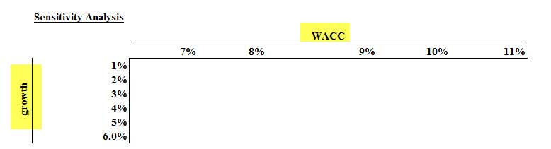
Step 1 – Create the Table Structure as given below

• Since we have two sets of assumptions – Cost of Capital (WACC) and Growth Rates (g), you need to prepare a table given below.
• You are free to switch the row and column inputs. Instead of WACC, you may have growth rates and vice-versa.

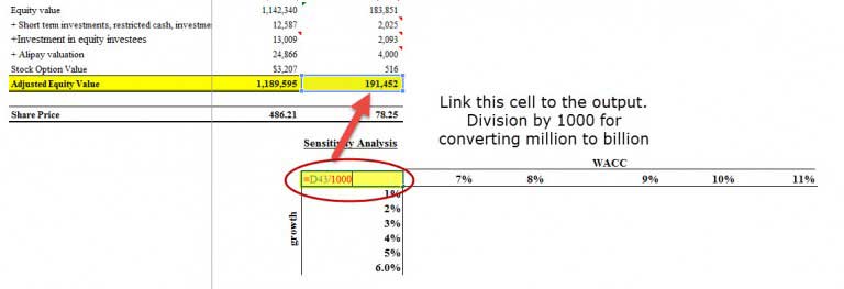
Step 2 – Link the Point of Intersection to the Output Cell.

The point of intersection of the two inputs should be used to link the desired output. In this case, we want to see the effect of these two variables (WACC and growth rate) on Equity value. Hence, we have linked the intersecting cell to the output.

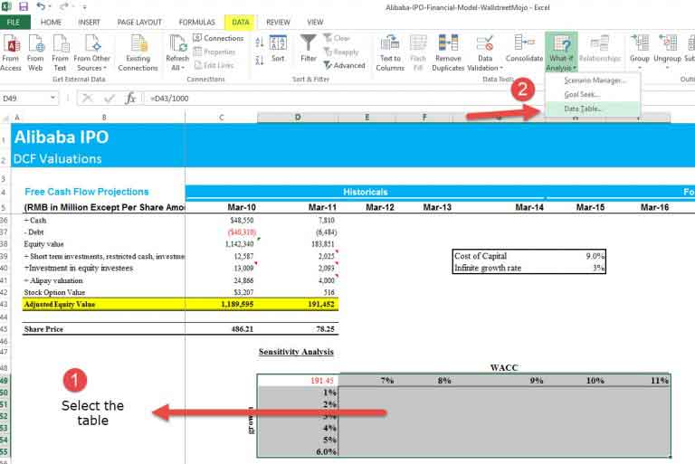
Step 3 – Open Two Dimensional Data Table

• Select the table that you have created
• Then click on Data -> What if Analysis -> Data Tables

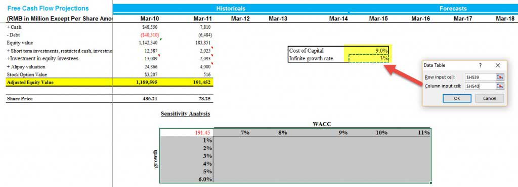
Step 4 – Provide the row inputs and column inputs.

• Row input is the Cost of Capital or Ke.
• The column input is the growth rate.
• Please remember to link these inputs from the original assumption source and not from inside the table.

Step 5 – Enjoy the output.

• Most pessimistic output values lie in the right-hand top corner, where the Cost of Capital is 11%, and the growth rate is only 1%
• The most optimistic Alibaba IPO Value is when Ke is 7%, and g is 6%
• The base case we calculated for 9% ke and 3% growth rates lies in the middle.
• This two-dimensional sensitivity analysis in the excel table provides the clients with an easy scenario analysis that saves a lot of time.

• The Goal Seek command is used to bring one formula to a specific value
• It does this by changing one of the cells that is referenced by the formula
• Goal Seek asks for a cell reference that contains a formula (the Set cell). It also asks for a value, which is the figure you want the cell to be equal
• Finally, Goal Seek asks for a cell to alter to take the Set cell to the required value

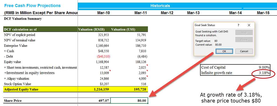
Let us have a look at the DCF of Alibaba IPO Valuation.

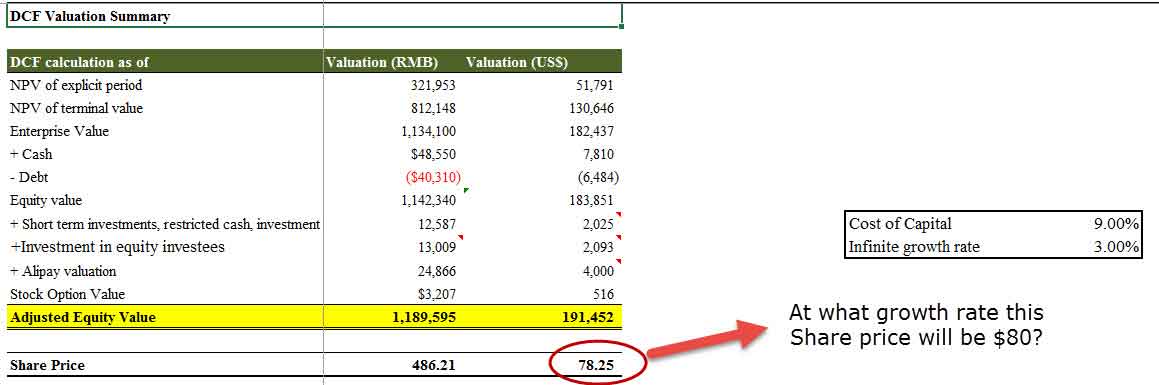
As we know from DCF that growth rates and valuation are directly related. Increasing growth rates increase the share price of the stock.

Let’s assume that we want to check at what growth rate will the stock price touches $80.

As always, we can do this manually by changing the growth rates to continue to see the impact on the share price. This will, again, be a tedious process. In our case, we may have to input growth rates many times to ensure that the stock price matches $80.

However, we can use a function like Goal Seek in excel to solve this in easy steps.

Step 1 – Click on the cell whose value you wish to set. (The Set cell must contain a formula)

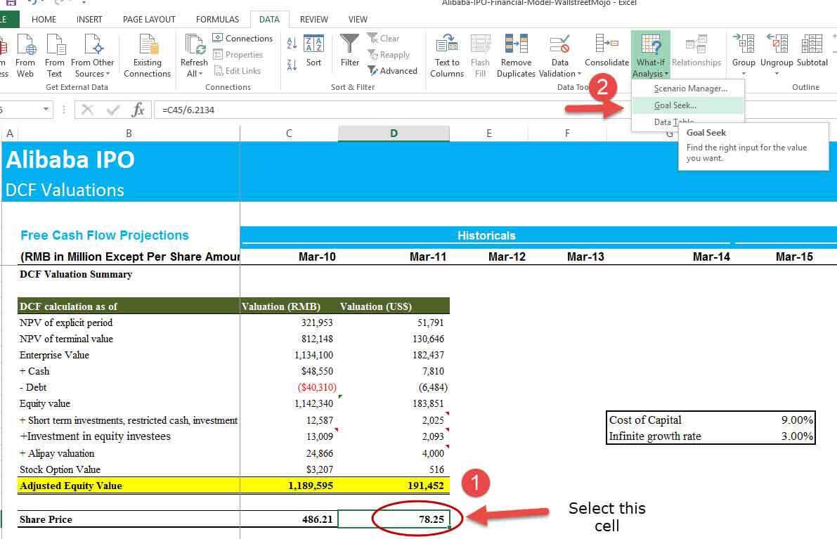
Step 2 – Choose Tools, Goal Seek from the menu, and the following dialog box appears:

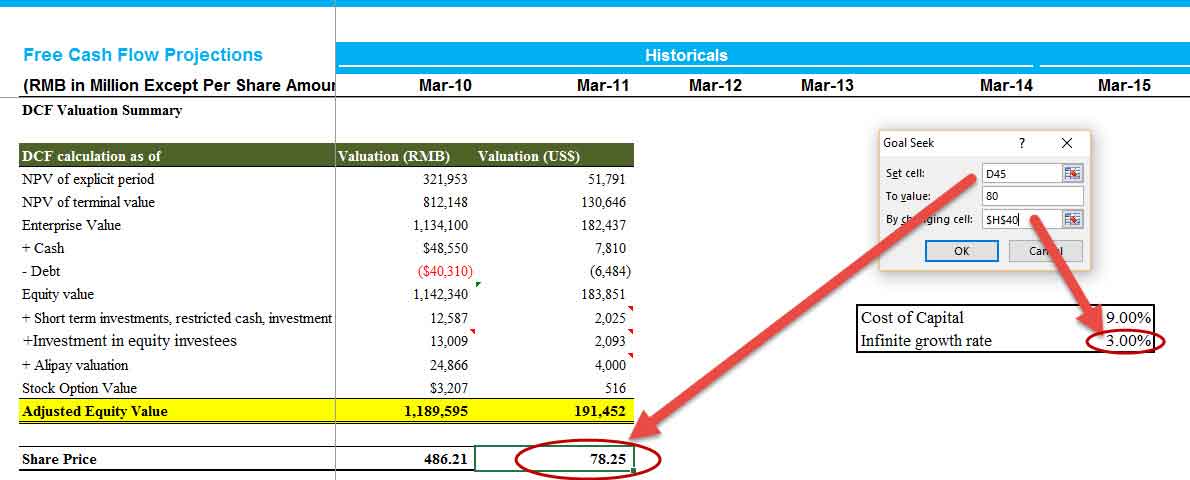
• The Goal Seek command automatically suggests the active cell as the Set cell.
• This can be over-typed with a new cell reference, or you may click on the appropriate cell on the spreadsheet.
• Now enter the desired value this formula should reach.
• Click inside the “To Value” box and type in the value you want your selected formula to equal.
• Finally, click inside the “By Changing Cell” box and either type or click on the cell whose value can be changed to achieve the desired result.
• Click the OK button, and the spreadsheet will alter the cell to a value sufficient for the formula to reach your goal.

Step 3 – Enjoy the output.

Goal Seek also informs you that the goal was achieved.

Sensitivity analysis in excel increases your understanding of the financial and operating behavior of the business. We learned from the three approaches – One Dimensional Data Tables, Two Dimensional Data Tables, and Goal Seek- that sensitivity analysis is extremely useful in finance, especially in the context of valuations – DCF or DDM.

You can develop cases to reflect valuation sensitivity to changes in interest rates, recession, inflation, GDP, etc., on the valuation. However, you can also get a macro-level understanding of the company and industry. Thought and common sense should be employed in developing reasonable and useful sensitivity cases.

If you learned something about Sensitivity Analysis in Excel, please leave a comment below. Let me know what you think. Many thanks, and take care. Happy Learning!