Rotate Pie Chart In Excel

Last Updated :

21 Aug, 2024

Blog Author :

Edited by :

Reviewed by :

Table Of Contents

What Is Excel Rotate Pie Chart?

Rotate Pie Chart in Excel is a feature that effectively displays many Pie Chart slices and proper layout tuning of the label to enhance slice visualization. We can separate the slices with space to differentiate them easily. Rotating supports avoiding the overlap of labels and chart titles and facilitating the considerable amount of empty area on each data label.

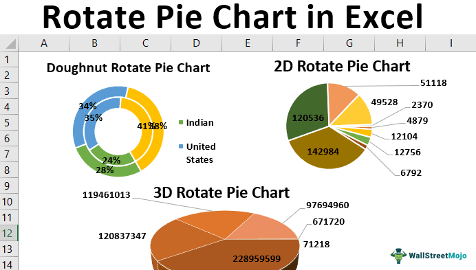
For example, we can apply the Rotate Pie Chart feature on different Pie chart types, as shown in the image below.

You are free to use this image on your website, templates, etc, Please provide us with an attribution link

What Is Excel Rotate Pie Chart?

Rotate Pie Chart in Excel is a feature that showcases tiny Pie Chart slices to enhance slice visualization.
If there are overlapping labels and chart titles, rotating facilitates the considerable amount of empty area on each data label.
The use of the camera tool in rotating the Pie Chart results in decreasing the resolution and changing the appearance of the object.
The doughnut Pie Chart is useful when two data series are presented. We can also use the Rotate option in the 2D & 3D Pie Chart types.

How To Rotate Pie Chart In Excel?

We can Rotate Pie Chart In Excel in a few ways, namely:

Changing the angle of the first Pie slice is presented in the series options.
From the quick access toolbar we can use the camera tool commands.

Using these options helps apply the rotation on the Pie Chart in Excel.

Excel Pie Chart Video Explanation

Download Template

This article must help understand Rotate Pie Chart in Excel with its formulas and examples. You can download the template here to use it instantly.

Examples

We will consider examples for different types of Pie Charts and apply the Rotate Pie Chart feature.

Example #1 - 2D Rotate Pie Chart

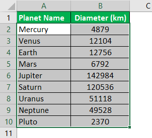
The creation of 2D rotates a pie chart on the diameter of nine planets in the solar system.

The steps to create a 2D Pie Chart and rotate it are,

Open the Excel worksheet.
Insert the data regarding the diameter of nine planets in the table format, as shown in the below-mentioned figure.
Select the data by pressing “CTRL+A” by placing the cursor anywhere in the table or selecting through the mouse.
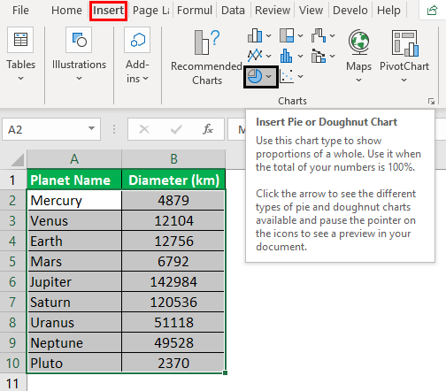
Go to the “Insert” tab on the ribbon. Next, move the cursor to the “Charts” area to select the “Pie Chart.”
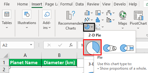
Click on the “Pie Chart”, select the “2-D Pie,” as shown in the figure, and develop a 2D Pie Chart.
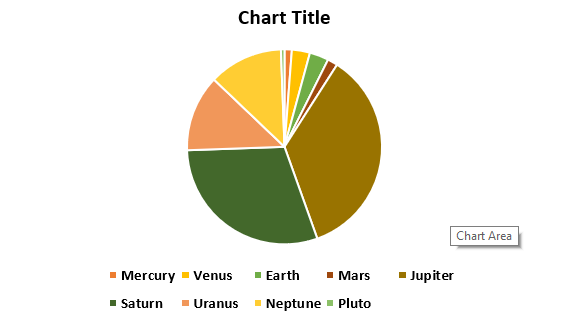
We get the following 2D Rotate Pie Chart.
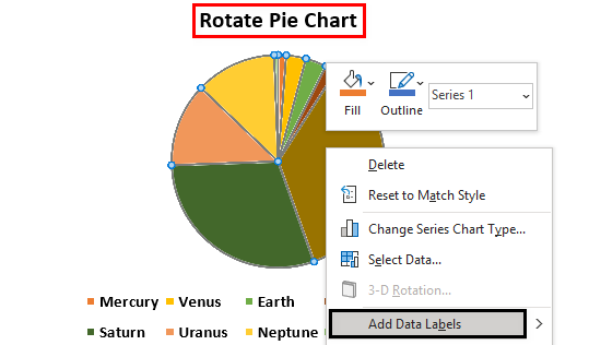
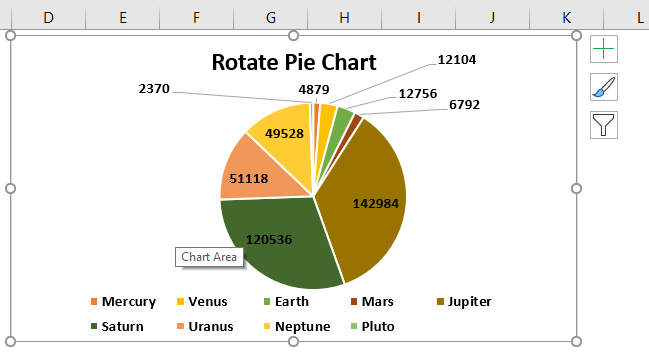
In the next step, change the chart’s title, and add data labels.
To rotate the Pie Chart, click on the chart area.
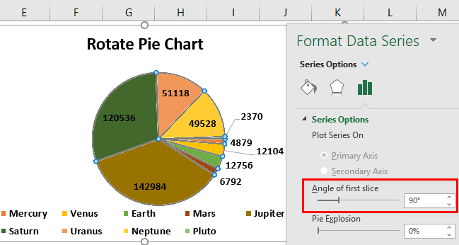
Right-click the Pie Chart, and select the “Format Data Series” option.
Change the angle of the first scale to 90 degrees to display the chart properly.

Now, the Pie Chart looks good, clearly representing the small slices, as shown below.

Example #2 - 3D Rotate Pie Chart

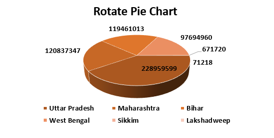
Creation of a 3D rotate Pie Chart on the population of various states in India.

The steps to create a 3D Pie Chart and rotate it are,

Step 1: Open the Excel worksheet.

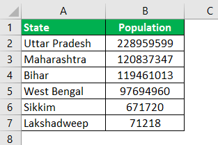
Step 2: Insert the data regarding the population of the Indian states in the table format in excel, as shown in the below-mentioned figure.

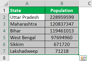
Step 3: Select the data by pressing “CTRL+A” by placing the cursor anywhere in the table or selecting through the mouse.

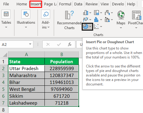
Step 4: Go to the “Insert” tab on the ribbon. Move the cursor to the “Chart” area to select the “Pie Chart.”

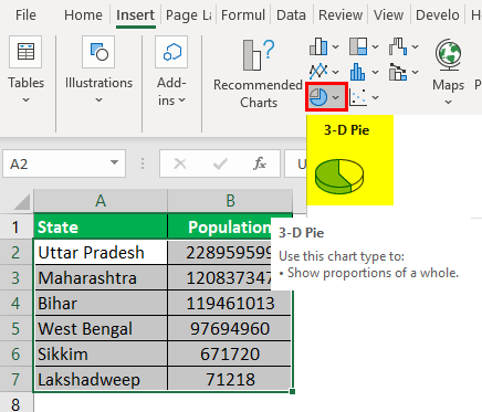
Step 5: Click the “Pie Chart”, select the “3-D Pie,” as shown in the figure, and develop a 3D Pie Chart.

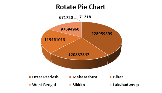
Step 6: In the next step, change the chart’s title and add data labels in the next step.

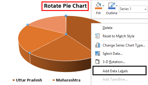
Then, the chart will look like this:

Step 7: Click the “Chart Area” to rotate the Pie Chart. Right-click the Pie Chart, and select the “Format Data Series” option.

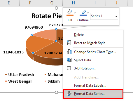
It opens the “Format Data Series” pane, as shown in the figure.

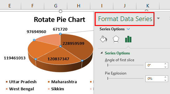
Step 8: Change the angle of the first scale to 90 degrees to display the chart properly.

Step 9: We get the following rotate Pie Chart.

Example #3 - Doughnut Rotate Pie Chart

Creation of a rotated Pie Chart for the doughnut chart in excel.

The steps to create a Doughnut Pie Chart and rotate it are,

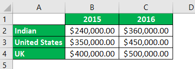
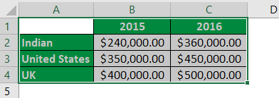
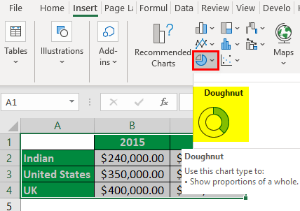
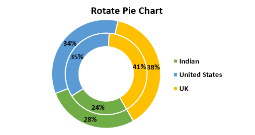
Step 1: Open the Excel worksheet. Insert the data regarding the sales made by a company in two years in different regions in the table format, as shown in the below-mentioned figure.

Step 2: Select the data by pressing “CTRL+A” by placing the cursor anywhere in the table or selecting through the mouse.

Step 3: Go to the “Insert” tab on the ribbon. Move the cursor to the “Chart” area to select the “Pie Chart.”

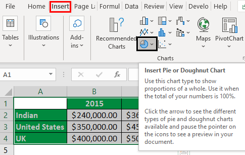
Step 4: Click on the “Pie Chart”, select the “Doughnut” chart, as shown in the figure, and develop the doughnut Pie Chart.

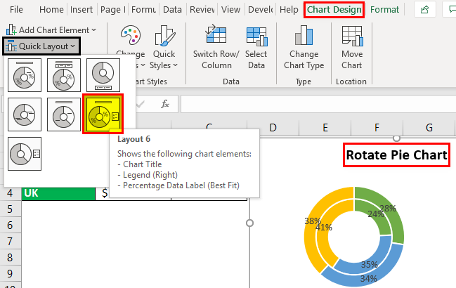
Step 5: In the next step, change the chart title, and select Layout 6 under the “Quick Layout” option to change the chart.

Step 6: Click on the “Chart” area to rotate the Pie Chart. Right-click the Pie Chart, and select the “Format Data Series” option.

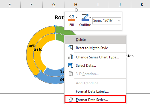
It opens the “Format Data Series” pane, as shown in the figure.

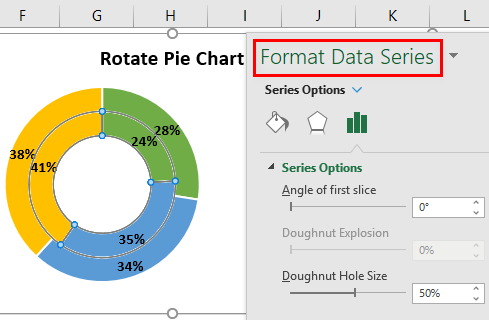
Step 7: Change the angle of the first scale to 150 degrees and change it to display the chart properly.

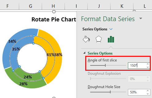
Step 8: We get the following doughnut to rotate the Pie Chart.

How To Use Rotate Pie Chart In Excel?

The Rotate Pie Chart has many uses, namely:

Changing the worksheet’s orientation to ensure the Pie Chart’s proper fit at the time of printing.
Modifying the location of the legend in the Pie Chart.
Reversing or changing the order of the slices in the Pie Chart.
Moving the individual labels of the Pie Chart.
Rotating the Pie Chart in various degrees, including 900, 1800, 2700, and 3600, in the clockwise and anti-clockwise directions.
Formatting the data series on the context menu of the Pie Chart.
Utilization of the camera tool effectively to apply the rotation on the chart from various angles.

Important Things To Note

Starting the rotation of the Pie Chart at 900 degrees is a good option.
The practice of starting to display the small parts of the Pie Chart at 12 o’clock is not right.

Frequently Asked Questions (FAQs)

1. What is the purpose of Rotate Pie Chart in Excel?

When we generate Pie Charts using the dataset, it might not be in the desired order we want. In such cases, to display or highlight the main data, we can use the rotate Pie Chart feature. It helps us to highlight important data on top or in the order we want.

2. What are the characteristics of Rotate Excel Pie Chart?

A few features of Rotate Excel Pie Chart are,
· We can rotate the chart to various degrees, including 900, 1800, 2700, and 3600, in the clockwise and anti-clockwise directions.
· Moving the individual labels of the Pie Chart for clear and readable display.
Reverse or change the order of the slices in the Pie Chart.

3. On which Pie Chart types can we use the Rotate feature?

We can use the Rotate options on all the Pie Chart types, such as Pie Chart, 2D Pie Chart, 3D Pie Chart, Doughnut Chart, etc.