Excel Table Styles & Formats

Excel Table Styles & Formats is a feature in Excel that is used on datasets in a worksheet to make it more presentable in a colorful or organized way.

Excel provides the Table Styles & Formats in Excel in various inbuilt formatting styles. However, we can create our own style formats and save them for future use.

For example, select a dataset, and press “Ctrl+T” to create a table for which we can add table styles. Then, click the “Table Design” tab, and select the desired style, as shown below.

The final table will look as shown in the above image.

• The Excel Table Styles & Formats is an amazing option in Excel to make the data more organized, presentable, or easily understood by the audience during a presentation.
• It helps us highlight the data as per our requirement, alternate rows from row 1, or we can start highlighting from the headers and then alternate the rows.
• We can copy the Excel Table Styles & Formats using the “Format Painter” option, and the “Conditional Formatting” option too.
• If the “Table Design” tab is not found on the ribbon,
  • Check if we have converted the initial dataset to a table using the “Ctrl+T” shortcut.
  • Ensure to click on any cell on the created table’s dataset to activate the tab.

We can create and format the table styles in Excel as follows:

• First, choose the entire dataset.

• Next, pressing the shortcut keys “Ctrl+T”.

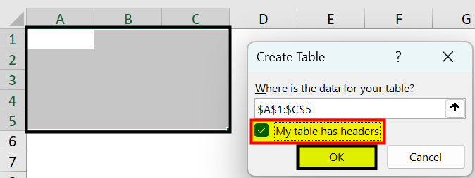
• The “Create Table” window appears with the selected cell range. Here, check/tick the “My table has headers” checkbox, and click “OK”, as shown below.

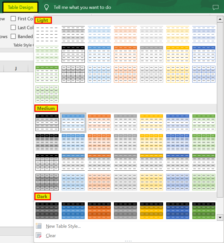
• Now, we will see a new tab, i.e., the “Table Design” tab on the Excel ribbon. So, select the “Table Design” tab → go to the “Table Styles” group → click the “Quick Styles” option drop-down, as shown below.

• Finally, select the table styles or the format as desired from the “Light, Medium, Dark” categories, as shown below.

We will consider some examples to create an excel table and format the table styles.

Example #1 - Creating the Table

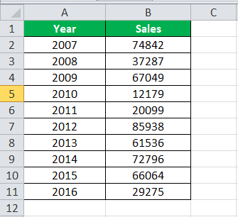
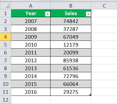
Let us start the process by creating the table. We have a simple sales table for ten years, given below.

The procedure to create a table are as follows:

First, place a cursor inside the data, and press the “Ctrl + T” (shortcut key to create tables). We will see a “Create Table” box, check/tick the box “My data has headers”, and click “OK”.

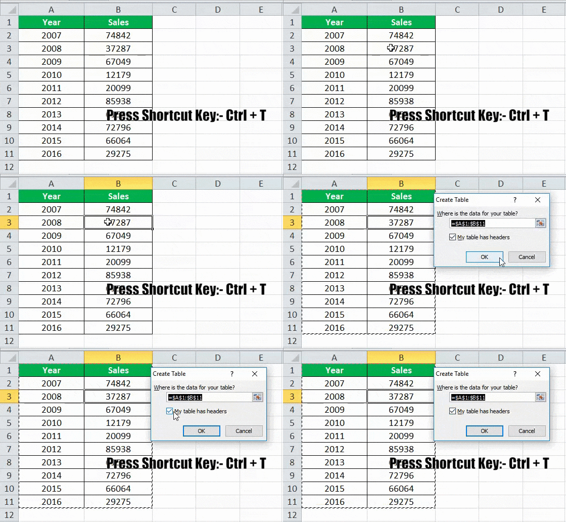
Now, we have our table created. It looks as shown below.

Example #2 - Change the Default Format of Table Style in Excel

Excel applied one of the default table styles in Excel. In Excel, we have many inbuilt table styles to select. We can change the existing table style to Excel at any time.

Example #3 - Create Your Own Table Format Style in Excel

We are not restricted from working with in-built table styles. Rather, we create our table style to satisfy ourselves. Under “New Table Style”, let us see how to design our new table style.

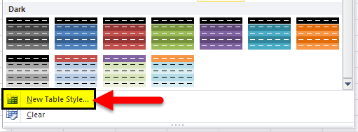
Now, we must click the “New Table Style”.

The “New Table Quick Style” window appears, as shown below.

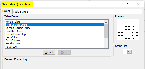
The first thing we need to do is to give a table name. Therefore, we have provided the name “My Table Style” in the “Name:” field, as shown below.

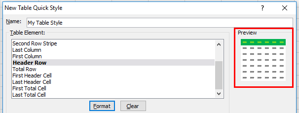
Under the “Table Element”, we must select the topic we want to modify. Here, we have chosen the “Header Row”, and then click the “Format” button, as shown below.

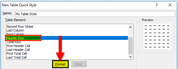
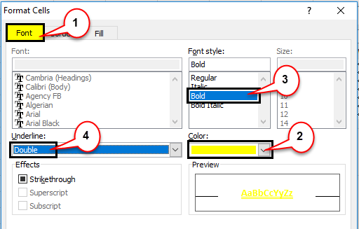
The “Format Cells” window appears. Here, select, “Font” as “yellow”, “Font Style” as “Bold”, and “Underline” as “Double”, or as per our desire, as shown below.

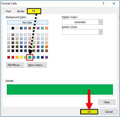
Next, we must go to the “Fill” tab, select the “Background Color:”, here, “Green”,and click “OK”.

Finally, we have created a style for our “Header Row”, and we can see the preview.

Under “Table Element”, select the “First Column.”

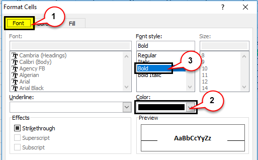
Again, click “Format.” Then, go to “Font”, choose the color “black,” and in “Font Style,” “Bold.”

We must go to “Fill”, select the “Background Color” as “light red”, and click “OK”.

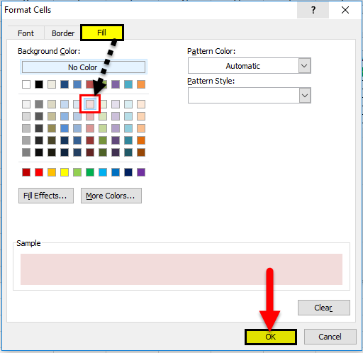
Now, we can see the preview.

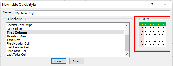
We have created our table format in Excel. Next, we must apply and see the table style in Excel. Then, under the “Design” tab, click on the drop-down list of “Table Styles.” Firstly, we may see the “Custom” table created, and select that table style.

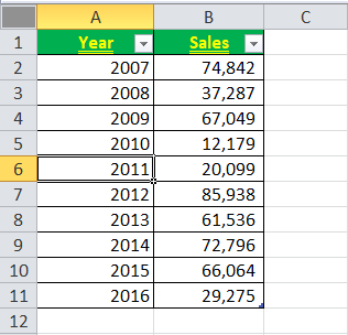
Now, we have applied our table format style in Excel, and our final table style is shown below.

• We must ensure that the “My data has headers” checkbox is ticked while creating a table.
• While designing our table style, we need to prepare each section separately.
• We can play with many formulas by applying the “Total Row” option.
• We must always give a table a name because it is easy to find which tables we are working on.