ABS Excel Function (Absolute)

The ABS Excel function is also known as the Absolute function, which calculates the absolute values of a given number. The negative numbers given as input are changed to positive numbers. If the argument provided to this function is positive, it remains unchanged.

ABS is a built-in function categorized under the Math/Trig function, which gives the absolute value of a number. It always returns a positive number.

For example, suppose you want to calculate the export and import of your company. If the export or import has positive and negative values, the Excel ABS function returns the absolute value of a number. The ABS function can convert negative numbers to positive numbers. Whereas the positive numbers and zero will be unaffected.

Arguments used in ABS Formula in Excel:

• number - The number you want to calculate the absolute value in Excel.

The number can be given as directed, in quotes, or as cell references. It can be entered as a part of an ABS formula in Excel. It can also be a Mathematical operation giving a number as an output. For example, in the function of ABS, if the supplied number argument is non-numeric, it provides #VALUE! Error.

Example #1

Suppose you have a list of values given in B3:B10, and you want the absolute values of these numbers.

For the first cell, you can type the ABS formula in Excel:

=ABS(B3)

Press the “Enter” key. As a result, it will return to 5.

You can drag it to the rest of the cells and get their absolute values in Excel.

All the numbers in C3:C10 are absolute.

Example #2

Suppose you have revenue data for the seven departments of your company, and you want to calculate the variance between the predicted and actual revenue.

For the 1^st one, you need to use the ABS formula in Excel:

=(D4-E4)/ABS(E4)

Now, press the “Enter” key. Subsequently, it will give 0.1667.

You can drag it to the rest of the cells to get the variance for the remaining six departments.

Example #3

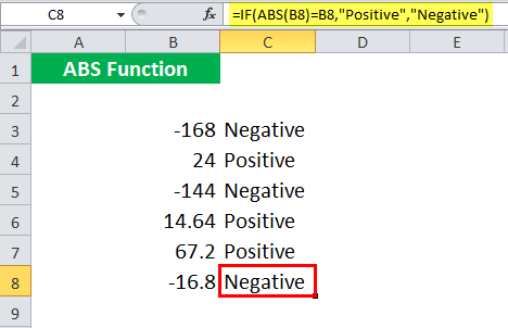
Suppose you have some data in B3:B8 and want to check which numbers are positive and negative. To do so, you can use the function of ABS to find absolute value in Excel.

You can use the ABS formula in Excel:

=IF(ABS(B3) = B3, “Positive”, “Negative”)

If B3 is a positive number, ABS(B3) and B3 will be the same.

Here, B3 = -168. So, it will return “Negative” for B3. Similarly, you can do this for the rest of the values.

Example #4

Suppose you have a list of predicted and actual data from an experiment. Now, you want to compare which of these lie within the tolerance range of 0.5. So, the data is given in C3: D10, as shown below.

To check which ones are within the tolerance range, you can use the ABS formula in Excel:

=IF(ABS(C4-D4) <= 0.5, "Accepted", "Rejected")

It is accepted if the Actual and Predicted difference is less than or equal to 0.5. Else, it is rejected.

For the first one, the experiment is rejected as 151.5 – 150.5 = 1, greater than 0.5.

Similarly, you can drag it to check for the rest of the experiments.

Example #5

Suppose you have a list of numbers and want to calculate the closest even number of the given numbers.

You can use the following ABS formula in Excel:

=IF(ABS(EVEN(B3) - B3) > 1, IF(B3 < 0, EVEN(B3) + 2, EVEN(B3) - 2), EVEN(B3))

If EVEN(B3) is the nearest EVEN number of B3, then ABS(EVEN(B3) – B3) is less than or equal to 1.

If EVEN(B3) is not the nearest EVEN number of B3, then

EVEN(B3) – 2 is the nearest value of B3 if B3 is positive

EVEN(B3) + 2 is the nearest value of B3 if B3 is negative

So, if ABS(EVEN(B3) – B3) > 1, then

If B3 < 0 i.e., if B3 is negative => The nearest even value is EVEN(B3) + 2

If B3 is not negative => The nearest even value is EVEN(B3) – 2

If ABS(EVEN(B3) - B3) ≤ 1, then EVEN(B3) is the nearest even value of B3.

Here, B3 = -4.8.

EVEN(B3) = -4

ABS((-4) – (-4.8)) gives 0.8

ABS(EVEN(B3) - B3) > 1 is FALSE, so it will return EVEN(B3).

Example #6

Suppose you want to identify the closest value of a list of values to a given value. You can do so using the ABS function in Excel.

The list of values you want to search for is provided in B3:B9; the lookup value is given in cell F3.

You can use the following ABS formula in Excel:

=INDEX(B3:B9, MATCH(MIN(ABS(F3 - B3:B9)), ABS(F3 - B3:B9), 0))

And, press CTRL + SHIFT + ENTER (or COMMAND + SHIFT + ENTER for MAC)

Please note that the syntax is an array formula, and simply pressing the ENTER key may give an error.

Let us see the ABS formula in detail:

• (F3 – B3:B9) will return an array of values {-31, 82, -66, 27, 141, -336, 58}
• ABS(F3 – B3:B9) will give the absolute values in Excel and returns {31, 82, 66, 27, 141, 336, 58}
• MIN(ABS(F3 – B3:B9)) will return the minimum value in the array {31, 82, 66, 27, 141, 336, 58} i.e., 27.
• MATCH(27, ABS(F3 – B3:B9), 0)) will look for the position of “27” in {31, 82, 66, 27, 141, 336, 58} and return 4.
• INDEX(B3:B9, 4) will give the value of the 4^th element in B3:B9.

It will return the closest value from the provided list of values B3:B9, i.e., 223.

You may notice that the curly braces have been automatically added to the entered ABS formula. For example, that happens when you insert an array formula.

• The ABS function returns a number's absolute value (modulus).
• The function of ABS converts negative numbers to positive numbers.
• In the function of ABS, positive numbers are unaffected.
• In the function of ABS, #VALUE! Error occurs if the supplied argument is non-numeric.

This article is a guide to ABS Function in Excel. Here, we learn how to use the ABS in Excel, along with Excel examples and downloadable Excel templates. You may also look at these useful functions in Excel: -

• Absolute Return
• Absolute Reference in Excel
• COUNTIF Formula in Excel
• COUNTIF Function with Multiple Criteria
• Excel Worksheet Tab