SUMPRODUCT in Excel

SUMPRODUCT Function in Excel

The SUMPRODUCT excel function multiplies the numbers of two or more arrays and sums up the resulting products. An array is a range of cells supplied as an argument to the SUMPRODUCT function. A product is the output of the multiplication of two numbers.

For example, a worksheet consists of numeric values in columns A and B. They are listed as follows:

Column A

• Cell A1 contains 3
• Cell A2 contains 4
• Cell A3 contains 5

Column B

• Cell B1 contains 2
• Cell B2 contains 6
• Cell B3 contains 1

The formula “=SUMPRODUCT(A1:A3,B1:B3)” returns 35. The given formula has calculated the output as (3*2)+(4*6)+(5*1)=35. Hence, the SUMPRODUCT multiplies the respective values of the specified arrays and sums up the resulting products.

Had there been only one range, A1:A3, the formula “=SUMPRODUCT(A1:A3)” would have returned 12. This is because, in case of one array, the SUMPRODUCT excel function returns the sum of the values of the single array.

Even though the SUMPRODUCT works on arrays, it does not require the CSE shortcut (Ctrl+Shift+Enter) to operate. Rather, the “Enter” key is pressed to perform the calculations.

The SUMPRODUCT function is categorized under the Math and Trigonometry functions of Excel. To extend the functionality of the SUMPRODUCT function, it can be combined with several other functions of Excel.

Syntax of the SUMPRODUCT Formula in Excel

The syntax of the SUMPRODUCT excel function is shown in the following image:

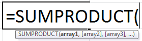
The SUMPRODUCT function accepts the following arguments:

• array1: This is the first array (range) whose values are to be multiplied and then added.
• array2: This is the second array (range) whose values are to be multiplied and then added.
• array3: This is the third array (range) whose values are to be multiplied and then added.

The “array1” argument is mandatory. The “array2,” “array3,” and the subsequent array arguments are optional.

Note: By default, the SUMPRODUCT function in excel multiplies numbers. However, it can also perform addition, subtraction, and division. For such arithmetic operations, place the relevant operator like “plus” (+), “minus” (-), or “forward slash” (/) between the array arguments supplied to the SUMPRODUCT function.

Video Explanation of SUMPRODUCT Excel Function

Sumproduct Excel Function Examples

Let us consider some examples to understand the working of the SUMPRODUCT function of Excel.

Example #1–Multiply and Add Numbers

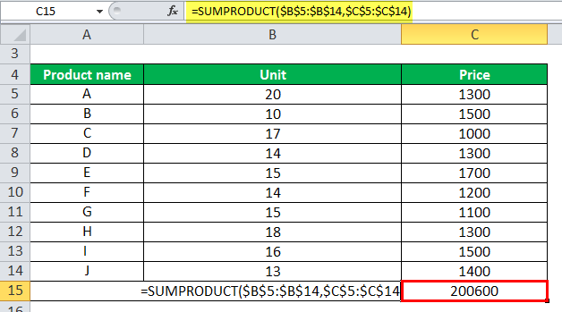
The succeeding image shows the prices (in $ in column C) and the number of units sold (column B) of 10 products. Calculate the total sales revenue generated by the products A to J.

Step 1: Enter the following formula in cell B15.

“=SUMPRODUCT($B$5:$B$14,$C$5:$C$14)”

Step 2: Press the “Enter” key. The output is $200,600. Hence, the total sales revenue generated by the given products (A to J) is $200,600.

For simplicity, we have shown the formula in cell B15 and given the result in cell C15.

Note: The absolute references (shown by the dollar symbol) in the SUMPRODUCT formula ensure that the formula does not change on being copied.

Explanation: The given SUMPRODUCT formula multiplies the values of column B with the corresponding values of column C. Thereafter, the products obtained are summed up.

The SUMPRODUCT formula (entered in step 1) works as follows:

(20*1300)+(10*1500)+(17*1000)+(14*1300)+(15*1700)+(14*1200)+(15*1100)+(18*1300)+(16*1500)+(13*1400)

=26000+15000+17000+18200+25500+16800+16500+23400+24000+18200

=200600

Hence, the output of the SUMPRODUCT formula is $200,600.

Example #2–Multiply and Add Based on a Criterion (Condition)

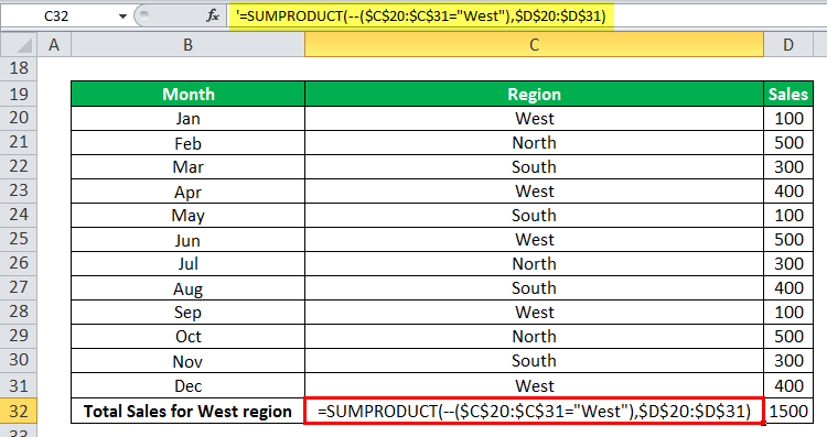
The succeeding image shows the sales revenue (in $ in column D) generated by the different regions (column C) for twelve months. Calculate the total sales revenue generated by the West region for the given period.

Step 1: Enter the following formula in cell C32.

“=SUMPRODUCT(--($C$20:$C$31="West"),$D$20:$D$31)”

Step 2: Press the “Enter” key. The output is $1,500. Hence, the total sales revenue generated by the West region for the period of twelve months is $1,500.

For simplicity, the SUMPRODUCT formula is shown in cell C32 and the result is given in cell D32.

Explanation: The formula $C$20:$C$31="West" returns a series of logical values, true or false. It returns true for all cells (of the range C20:C31) that contain “West.” For cells containing values other than “West” (like North or South), the formula returns false.

The unary operator or the double negative symbol (--) converts the true and false values into 1 and 0 respectively. Had we not used the unary operator, the SUMPRODUCT function in excel would have treated the non-numeric values (of column C) as zeroes.

The first array of the SUMPRODUCT function results from the formula $C$20:$C$31="West". This array consists of only ones (1) and zeroes (0). The second array of the SUMPRODUCT function is $D$20:$D$31.

Since all cells (of the range C20:C31) containing “West” evaluate to 1, the SUMPRODUCT excel function works as follows:

(1*100)+(0*500)+(0*300)+(1*400)+(0*100)+(1*500)+(0*300)+(0*400)+(1*100)+(0*500)+(0*300)+(1*400)

=100+0+0+400+0+500+0+0+100+0+0+400

=1500

Hence, the output of the SUMPRODUCT formula is $1,500.

Example #3–Mutliply and Add to Find the Weighted Average

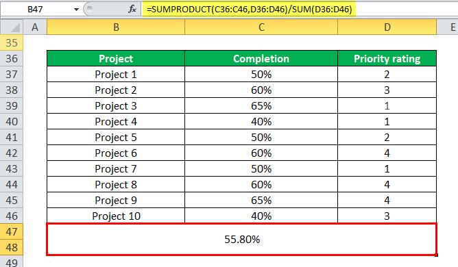
The succeeding image shows the completion percentages (column C) of 10 projects of an organization. With these percentages, one can figure out the extent to which the respective project has been completed. The priority rating (column D) is the weight assigned to a project.

Calculate the weighted average of the given projects with the help of the SUMPRODUCT excel function.

Step 1: Enter the following SUMPRODUCT formula.

“=SUMPRODUCT(C36:C46,D36:D46)/SUM(D36:D46)”

Step 2: Press the “Enter” key. The output is 55.8%. Hence, the weighted average is 55.8%.

Explanation: For calculating the weighted average, the following calculations are performed in the given sequence:

1. The completion percentages (C36:C46) are multiplied by the weights (D36:D46).
2. The resulting products (obtained in step a) are added.
3. The answer obtained (in step b) is divided by the sum of the weights .

The SUMPRODUCT formula (entered in step 1) works as follows:

/(0+2+3+1+1+2+4+1+4+4+3)

=(0+1+1.8+0.65+0.4+1+2.4+0.5+2.4+2.6+1.2)/25

=13.95/25

=0.558 or 55.8%

Hence, the weighted average is 55.8%.

Note: The non-numeric values in cells C36 and D36 are treated as zeroes by the given SUMPRODUCT formula.

Example #4–Multiply and Add Based on Multiple Criteria (Conditions)

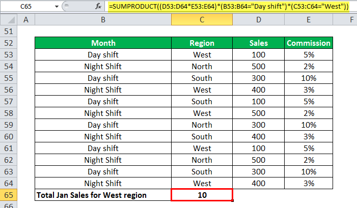
The succeeding image shows the sales revenues (in $ in column D) generated by the employees of different regions (column C). On every sale, a percentage of commission (column E) is earned by the employees.

Further, the employees work in two shifts, the day shift and the night shift. The entire dataset relates to the month of January of a particular year.

Calculate the total commission (in $) paid to the employees of the West region who are working in day shifts.

Step 1: Enter the following formula in cell C65.

“=SUMPRODUCT((D53:D64*E53:E64)*(B53:B64="Day shift")*(C53:C64="West"))”

Step 2: Press the “Enter” key. The output is $10.

Explanation: The formula B53:B64="Day shift" helps find the cells (in the range B53:B64) that contain the words “day shift.” If a cell of column B contains “day shift,” the result is true. Otherwise, the result is false.

Likewise, the formula C53:C64="West" returns true or false depending on the value of cells in the given range (C53:C64). It returns true for all cells of column C that contain “West.” If the cells contain values other than “West” (like North or South), this formula returns false.

Since there is no unary operator (--) preceding these formulas, the true and false values are not converted into binary digits (0 and 1).

The SUMPRODUCT formula (entered in step 1) consists of multiple criteria. The criteria for columns B and C are “day shift” and “West” respectively. From the given dataset, only rows 53 and 61 satisfy the stated criteria.

Therefore, the SUMPRODUCT excel formula multiplies and adds the corresponding values of columns D and E for rows 53 and 61 only.

Row 53 contains 100 and 5% in cells D53 and E53 respectively. Likewise, row 61 also contains 100 and 5% in cells D61 and E61 respectively. These numbers are multiplied and then added.

The SUMPRODUCT formula works as follows:

(100*5%)+(100*5%)

=10

Hence, the employees working in day shifts and belonging to the West region are paid a total commission of $10.

The Properties of the SUMPRODUCT Excel Function

The features of the SUMPRODUCT excel function are listed as follows:

• The minimum number of arrays to be supplied to the SUMPRODUCT function is 1. If a single array is supplied, the function returns the sum of all the items of this array.
• The maximum number of arrays that can be specified is 255 in Excel 2007 and the newer versions. In the older Excel versions, the maximum limit of arrays is fixed at 30.
• All array arguments must have the same number of rows and columns. If not, the SUMPRODUCT function returns the #VALUE error.
• The SUMPRODUCT excel function treats the non-numeric entries of an array as zeroes.
• The logical tests within arrays evaluate to the Boolean values, true or false. These values can be converted to 1 and 0 with the help of the unary operator (--).

Note: The SUMPRODUCT can be used as a VBA function. For instance, a code can be created as follows:

Sub ABC()
MsgBox Evaluate("=SUMPRODUCT(($A$1:$A$5=""Tanuj"")*($B$1:$B$5))")
End Sub

The values of array A1:A5 that evaluate to “Tanuj” are multiplied by the corresponding values of the array B1:B5. The resulting products are then summed up.

Frequently Asked Questions

Recommended Articles

This has been a guide to SUMPRODUCT in Excel. Here we discuss how to use SUMPRODUCT Function along with step by step excel example.. You may also look at these useful functions of Excel-

• SUMPRODUCT with Multiple Criteria
• SUBTOTAL Excel Function
• AGGREGATE Function
• SIGN Excel Function
• Redo Shortcut in Excel