Table Of Contents
What Is N Excel Function?
The N Excel function is an inbuilt Information function that converts the given value into a number. The function can take numeric values, dates, logical values and texts as input.
Users can use the N() to show a comment in a formula, convert texts and special characters into zero, and logical TRUE and FALSE into 1 and 0, respectively.
For example, the following dataset lists values.
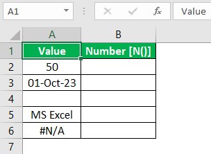
The aim is to convert the column A values into numbers and display the output in column B.
Then, we can use the formula N Excel in each target cell to achieve the required output.
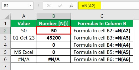
In the above formula N Excel example, the N() in each target cell accepts the cell reference to the value in the corresponding row to return the value as a number.
The output shows that the N() returns the input number as is since the input value is a number. But if the input value is a date, the function returns the date’s serial number equivalent.
On the other hand, the function output is a zero when the input value is a text or an empty cell.
Finally, if the input is an error value, the function returns the specified error value as the output.
Table of contents
- The N Excel Information function accepts a value and converts the value into a number. Typically, the function input can be numeric values, dates, text, special characters, and logical values.
- Users can use the Excel N function to convert non-numeric data into zero, add comments in formulas, and change Boolean data into 1s and 0s.
- The Excel N function accepts one mandatory argument, value, as the input. The argument can be a value, reference, or a formula.
- While we can use the Excel N function as a standalone function, using it with other inbuilt functions, such as the IF, SUM, and SUMPRODUCT, yields productive outcomes.
Syntax
The N() syntax is as follows:

Where,
- value: The value we aim to convert into a number.
The N() argument is mandatory, and it can be a value, reference to a value or formula returning a value.
Furthermore, the following table shows the list of possible N() inputs and their corresponding output values.
| Input Value | N() Output |
|---|---|
| A number | Same number without formatting. |
| A valid date | The date’s serial number. |
| TRUE | 1 |
| FALSE | 0 |
| An error value (#VALUE, #DIV/0!, #N/A, etc.) | Same error value |
| Other values | 0 |
How To Use N Excel Function?
We can use the N Excel function in two ways:
- Access the function from the Excel ribbon.
- Enter the function into the worksheet manually.
Method #1 – Access The Function From The Excel Ribbon
Choose a cell for output - The Formulas tab - The More Functions group down arrow - The Information function group right arrow - Find N Excel function from the listed functions and click it to select it.
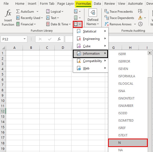
The Function Arguments window will open. Update the argument in the Value field.
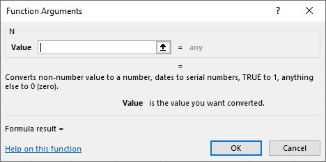
Finally, click OK in the Function Arguments window to view the N() output in the target cell.
Method #2 – Enter The Function Into The Worksheet Manually
- Select a cell to display the output.
- Type =N( in the cell.
- Enter the argument as a value, reference, or formula, and close the brackets.
- Press Enter to execute the N() and view the value converted into a number.
Examples
The following examples show the scenarios where we can use the N Excel function.
Example #1 - Converting A Date Into A Number
The following dataset lists students and their project submission dates.
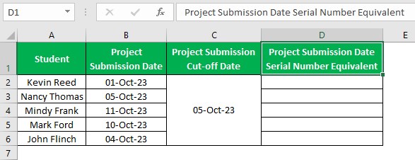
The task is to display the serial number equivalent of the project submission dates of students who submitted the projects on or before the cut-off date. Otherwise, the message “Project Submission Date Missed" should be the output. Assume the target cells are in column D.
Then, we can use the IF N Excel functions-based formula in the target cells to obtain the required output.
Step 1: Choose cell D2 and enter the following formula.
=IF(B2<=$C$2,N(B2),"Project Submission Date Missed.")
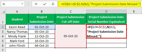
Step 2: Press Enter to view the formula output in the target cell.
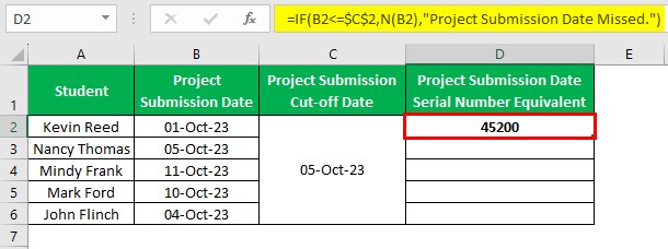
Step 3: Using the Excel fill handle, implement the formula in the remaining target cells.
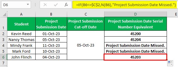
Let us check the cell D6 formula to understand its logic.
First, the Excel IF function condition checks if the cell B6 date value is smaller or equal to the cell C2 cut-off date. Since the specified project submission date in cell B6 falls before the cut-off date in cell C2, the IF condition holds. Thus, the IF() returns the TRUE value, which is the N().
The N() accepts the project submission date in cell B6 as the input and returns the specified date’s serial number equivalent, which the IF() returns as the required output, 45203.
Example #2 - Converting Text To Zero
The following dataset contains a list of fruits and their quantities.
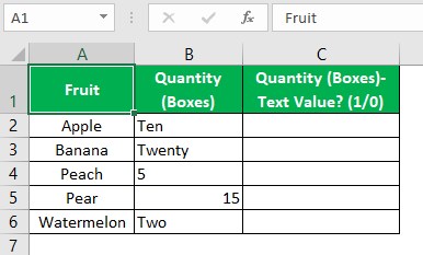
The aim is to check whether the fruit quantities are text values or not. If the quantity is a text value, the output must display as 0 and 1 otherwise. Assume the target cells are in column C.
Then, here is how to use the N Excel function with the IF() in each target cell to obtain the required output.
Step 1: Choose cell C2, enter the following formula, and press Enter.
=IF(N(B2)=0,0,1)
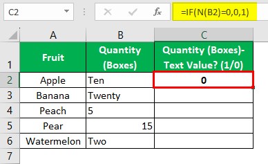
Step 2: Press Enter to view the formula output in the target cell.
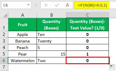
First, the N() accepts the cell reference to the quantity value in the corresponding row. Since the input value is a text, the N() returns the value of 0.
Next, the IF() condition checks of the N() output equals 0. Since the condition holds, the IF() returns the TRUE value, 0, as the output.
Please note that cells B4 and B5 show numbers, and yet the N() output values in cells C4 and C5 are different. The reason is that cell B4’s data format is Text, implying the value of 5 is a text. So, the N() output is 0.Thus, the IF() condition in the corresponding target cell holds, leading to the function returning the TRUE value of 0.
On the other hand, the value of 15 in cell B5 is indeed a number. So, the N() output is 15. Thus, the IF() condition in the corresponding target cell does not hold, leading to the function returning the FALSE value of 1.
Example #3 - Checking A Value With Data Validation
The following dataset lists a firm’s branch offices.
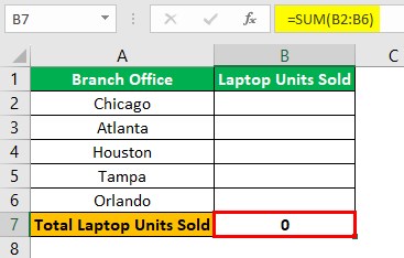
The user must update the laptop units sold data for each branch office in column B cells, and cell B7 sums the values in the range B2:B6 to give the total laptop units sold value.
However, we must ensure the user enters only numbers in the range B2:B6 so that the cell B7 SUM Excel function does not return an error value.
Then, we can use the N Excel function with the Data Validation feature to achieve the required data.
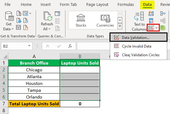
Step 1: Choose cells B2:B6 and Data - Data Validation - Data Validation.
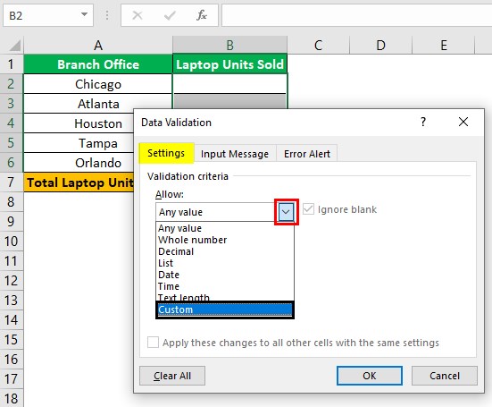
Step 2: The Settings tab in the Excel Data Validation window will open, where we must click the Allow field drop-down button to choose the Custom option.
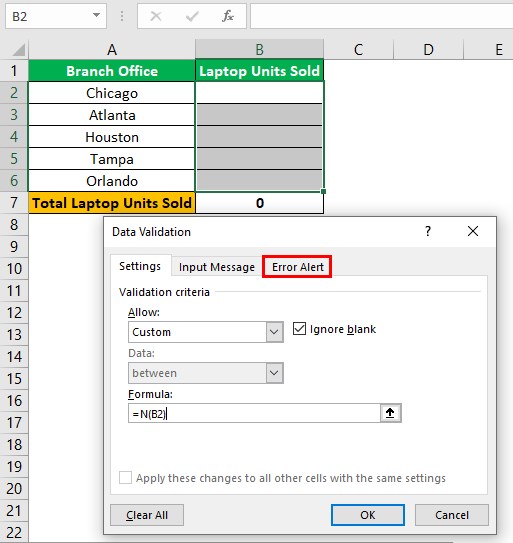
Next, enter the N() with reference to the first cell in the specific range, cell B2, as the Formula field value and click the Error Alert tab to open it.
Step 3: Update the Title and Error message fields according to the requirements.
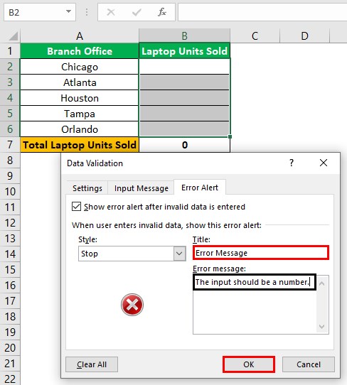
Next, click OK in the Data Validation window.
Step 4: Start typing the required numbers in the range B2:B6.
Assume we enter “Five” instead of the number 5 in cell B4.
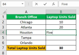
Pressing Enter will show the Error Message box with the error message we specified in the Error Alert tab within the Data Validation window.
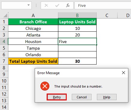
Step 5: Click Retry in the Error Message box to get the cursor inside the issue cell B4.
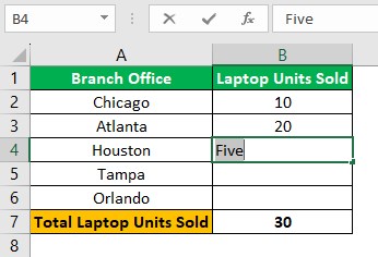
Step 6: Enter the correct number value in cell B4 and the remaining cells B5:B6.
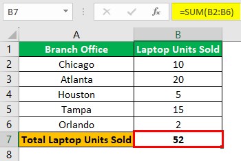
Finally, once we update the required numbers in the range B2:B6, cell B7 containing the SUM() will show the sum of the entered values as the required total laptop units sold value.
Example #4 - Leaving Comment In Formula
The dataset below contains an employee’s monthly attendance data.
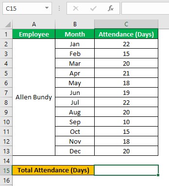
The task is to determine the employee’s total attendance based on the given monthly attendance data in the range C2:C13 and display the output in cell C15.
Then, we can use the SUM() in the target cell to achieve the required data.
However, we must include a comment in the cell C15 formula to inform the user that the value is the sum of the employee’s monthly attendance. Also, the comment must not be visible in the target cell and must not affect the SUM() output.
Then, we can use the SUM N Excel functions-based formula in the target cell instead of the SUM().
Step 1: Choose cell C15, enter the following formula, and press Enter.
=SUM(C2:C13)+N("Sum Of Allen Bundy's Monthly Attendance.")
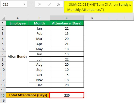
Firstly, the SUM() accepts the cell range C2:C13 containing the monthly attendance values as input, and it adds the values to return the total attendance, 220.
Next, we add the N() to the SUM() output, with the required comment supplied as input to the N(). Since the N() returns zero when the input value is text, the function returns zero in this case. So, the SUM N Excel functions-based formula returns the SUM() output, 220 days, as the required total attendance value in the target cell C15.
Thus, using the N() with the SUM() ensures that the comment is visible only in the Formula Bar when we select the target cell, with the target cell displaying the required value.
Example #5 - Counting Cells With More Than N Characters
The following dataset lists quotes by famous personalities.
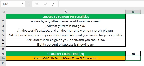
The aim is to count cells with more than 50 characters in the range A2:A7 and display the output in cell B10.
Then, we can use the N Excel function with the SUMPRODUCT and LEN excel functions in the target cell to achieve the required count.
Step 1: Choose cell B10, enter the following formula, and press Enter.
=SUMPRODUCT(N(LEN(A2:A7)>B9))
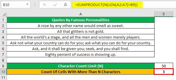
First, the Excel LEN function determines the total characters in each cell in the range A2:A7 to return an array of numbers {46;30;66;79;57;40}. Next, the formula compares each array element with the cell B9 value, 50, to determine the bigger value.
The array shows that the cells in the range A4:A6 contain more than 50 characters, while cells A2, A3, and A7 contain less than 50 characters. So, we get an array of TRUEs and FALSEs, {FALSE;FALSE;TRUE;TRUE;TRUE;FALSE}. The array element is TRUE if the corresponding array element in the LEN() output is greater than the character limit of 50, specified in cell B9. Otherwise, the array element is FALSE.
Next, the N() accepts the array of TRUEs and FALSEs to return an array of 1s and 0s, {0;0;1;1;1;0}. Finally, the Excel SUMPRODUCT function returns the sum of the products of the given array, 3, as the required count of cells containing more than 50 characters.
N Function Vs T Function
The differences between the N Excel function and Excel T function are as follows:
- Excel Inbuilt Function Group
While the N() falls under the Information Excel inbuilt function group, the T() belongs to the Text Excel inbuilt function group.
- Definition
The N() translates the specified value into a number. On the other hand, the T() determines if the specified value is a text.
- Function Return Value
When the input is a number, the N() output will be the number itself. If the input is a logical value, the output will be 1 for TRUE and 0 for FALSE. For the remaining data types, the function output will be 0.
On the other hand, when the input is a text, the T() output will be the text itself. For the remaining data types and logical values, the function returns an empty string.
- Primary Functionality
While the aim of using the N() is to convert values into numbers, we use the T() to distinguish between text-formatted data and other data types.
Important Things To Note
- The N Excel function returns the same number and error value supplied as the input to the function.
- If the input value to the N function is a valid date, the function returns the date’s serial number equivalent.
- The N function output is 1 when the input to the function is the Boolean TRUE and 0 when the input to the function is the Boolean FALSE.
- When the input to the N function is a text or any other data type that is non-numeric, the function output is 0.
Frequently Asked Questions (FAQs)
The N Excel works for logical values, as explained below with an example.
The following image shows two datasets. While the first one lists two value sets, the second shows the two logical values in Excel.
The task is to check if Value 1 exceeds Value 2 in each row and display the output as 1 or 0, where 1 indicates the condition holds and 0 indicates the condition is false. Assume the target cells are C2:C3.
Then, the steps are as follows:
Step 1: Choose cell C2, enter the N(), and press Enter.
=N(A2>B2)
Next, using the fill handle, update the formula in cell C3.
The N() in each target cell checks if the first value exceeds the second. If the condition holds, the output is TRUE. So, the N() converts the logical TRUE value into a number, 1, to return it as the output. On the other hand, if the condition is false, the output is FALSE. So, the N() converts the logical FALSE value into a number, 0, to return it as the output.
Furthermore, we shall see how the N() works when we supply the logical values directly, as cell references, or within double quotes.
Step 2: Choose cell C6, enter the N(), and press Enter.
=N(A6)
Next, using the fill handle, implement the formula in cell C7.
Step 3: Choose cell D6, enter the N(), and press Enter.
=N(TRUE)
Next, choose cell D7, enter the N(), and press Enter.
=N(FALSE)
Step 4: Choose cell E6, enter the N(), and press Enter.
=N("TRUE")
Next, choose cell E7, enter the N(), and press Enter.
=N("FALSE")
The output in the second dataset shows that when we supply the logical values directly or as cell references to the N(), the function converts the logical TRUE and FALSE into 1 and 0.
However, when we supply the logical values as texts to the N(), the function returns 0.
The important characteristics of N Excel function are as follows:
• If the input value to the N() is Boolean data, the N() converts them into 1s and 0s.
• The N() returns the input value as is if the specified value is a number or an Excel error value.
• If the input value supplied to the N() is a text, the N() output is 0.
The N Excel does not affect numerical values or errors.
When the input value supplied to the N() is a number or error value, the function returns the same number or error value as the function output.
However, in the case of a numeric value as input, the function returns the number without any formatting.
Download Template
This article must be helpful to understand the N Excel, with its formula and examples. You can download the template here to use it instantly.
Recommended Articles
This has been a guide to What Is N Excel. We learn the N Excel function syntax, how to use it with examples, and difference between N & T Excel functions. You can learn more from the following articles –
