MROUND in Excel

Last Updated :

21 Aug, 2024

Blog Author :

Edited by :

Reviewed by :

Table Of Contents

MROUND Function in Excel

The MROUND is the MATH and TRIGONOMETRY function in Excel and is used to convert the number to the nearest multiple numbers of the given number. For example, =MROUND(50,7) will convert the number 50 to 49 because the number 7 is the nearest multiple of 49. In this case, it has rounded down to the closest value. Similarly, if the formula is =MROUND(53,7), this will convert the number 53 to 56 because multiple numbers 7 nearest the number for number 53 is 56. Again, in this, it has rounded up to the nearest multiple values odd number 7.

MROUND Function in Excel

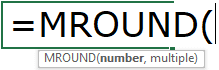
Syntax

Number: What is the number we are trying to convert to?
Multiple: The multiple numbers we are trying to round the Number.

Here, both the parameters are mandatory. Furthermore, both the parameters should include numerical values. Finally, we will practically see some examples of the MROUND function.

Examples to use MRound Function in Excel

Example #1

The MROUND Excel function rounds the number to the nearest multiple of the provided number. You must be thinking about how Excel knows whether to round up or round down. It depends on the result of the division.

For an example 16 / 3 = 5.33333, here decimal value is less than 0.5 so result of nearest multiple value of number 3 is 5, so 3 * 5 = 15. Here, Excel rounds down the value if the decimal value is less than 0.5.

Similarly, look at this equation 20 / 3 = 6.66667. In this equation, the decimal value is greater than 0.5, so Excel rounds up the result to 7, so 3 * 7 = 21.

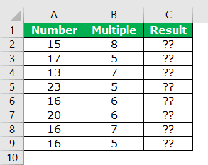
So for this example, consider the below data.
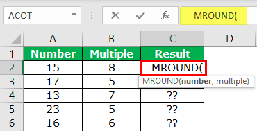
We must open Excel MROUND function in cell C2 first.
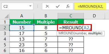
Select cell A2 value as the "Number" argument.
The second argument, "Multiple," is the cell B2 value.
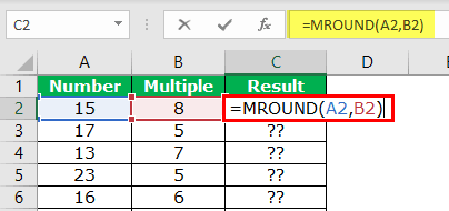
Press the "Enter" key. Then, copy and paste the formula to other cells to get the result.
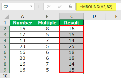
We got the result in all the cells. Let us look at each example individually now.

In the first cell, the equation reads 15/8 = 1.875. Since the decimal value is >= 0.5, Excel rounds up the number to the nearest integer value is 2. So here, multiple numbers are 8, and the resulting number is 2, so 8 * 2 = 16.

Look at the second equal 17/5 = 3.4. Here, the decimal is less than 0.5, so Excel this time rounds down the number to 3, and the result is 5 * 3 = 15.

Like this Excel, the MROUND function rounds down or rounds up the number to the nearest integer value of multiple numbers.

Example #2

We have seen how the MROUND function works. Now, we will see how we can apply the same to round up or down the time to the nearest multiple values.

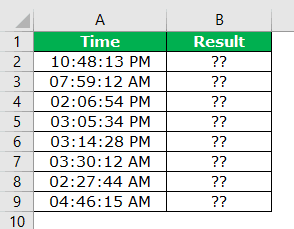
We will convert the time from the above timetable to the nearest 45-minute intervals. Below is the formula.

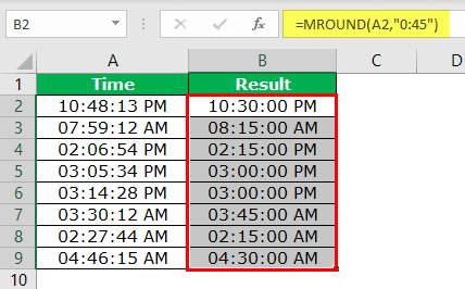
In this example, we have supplied the multiple values as "0:45." Therefore, it will be automatically converted to the nearest number, "0.03125". So, the number "0.03125" is equal to 45 minutes when we apply the time format to this number in Excel.

Things to Remember

Both the parameters should be numbers.
If anyone's parameter is not numeric, we will get the "#NAME?" error value.
Both the parameters should have the same signs, either positive or negative. We will get the "#NUM!" error value if both signs are supplied in a single formula.