SUMIF with Multiple Criteria in Excel
The SUMIF (SUM+IF) with multiple criteria sums the cell values based on the conditions provided. The criteria are based on dates, numbers, and text. The SUMIF function works with a single criterion, while the SUMIFS function works with multiple criteria in excel.
How to use SUMIF with Multiple Criteria?
The SUMIF function with multiple criteria is SUMIF(range, criteria, sum_range).
The following operators are used in the criteria argument:
- Comparison operators
- Greater than (>), less than (<), greater than or equal to (>=), less than or equal to (<=)
- Equal to (=), not equal to (<>)
- Wildcard characters
- Asterisk (*) [implies any number of characters]
- Question mark (?) [implies a single character]
Let us consider a few examples to understand SUMIF with multiple criteria.
#1–Text Criteria (Exact Match)
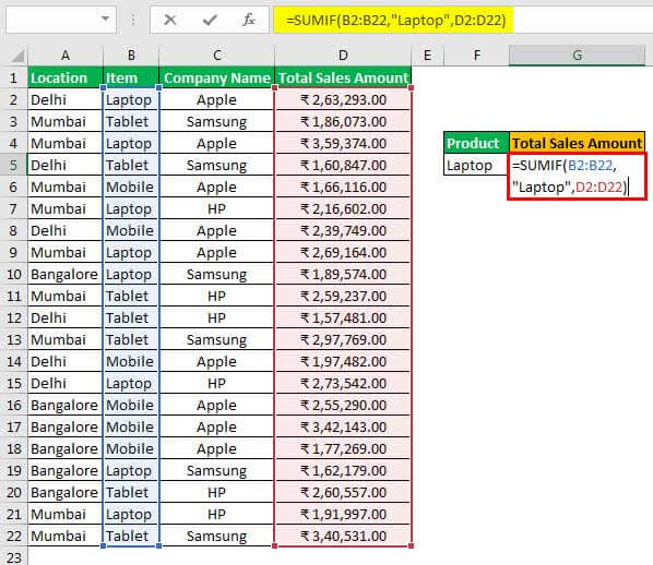
The following table contains the item sales for a particular location of an organization. We want to sum the laptop sales of the organization.

The steps to sum the laptop sales are listed as follows:
- Enter the formula shown in the following image.
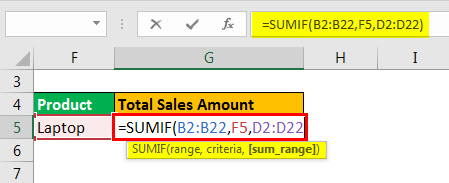
The range B2:B22 (column “item”) is compared with the criteria “laptop.” The sum_range is D2:D22 (column “total sales amount”)

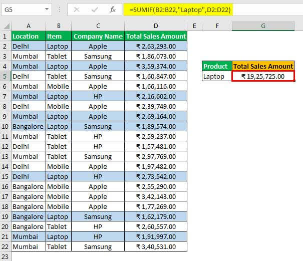
- Press the “Enter” key and the output appears, as shown in the following image.

#2–Text Criteria With Drop-Down List
The unfamiliar users of MS Excel usually do not use the formula given in “step 1” of “example #1.” The word “laptop” is directly specified in the “criteria” argument of the formula.
Alternatively, the cell reference can be given. The value in the referenced cell may be keyed or selected from the drop-down list.
Working on example #1, let us create a drop-down list to sum laptop sales. The steps are given as follows:
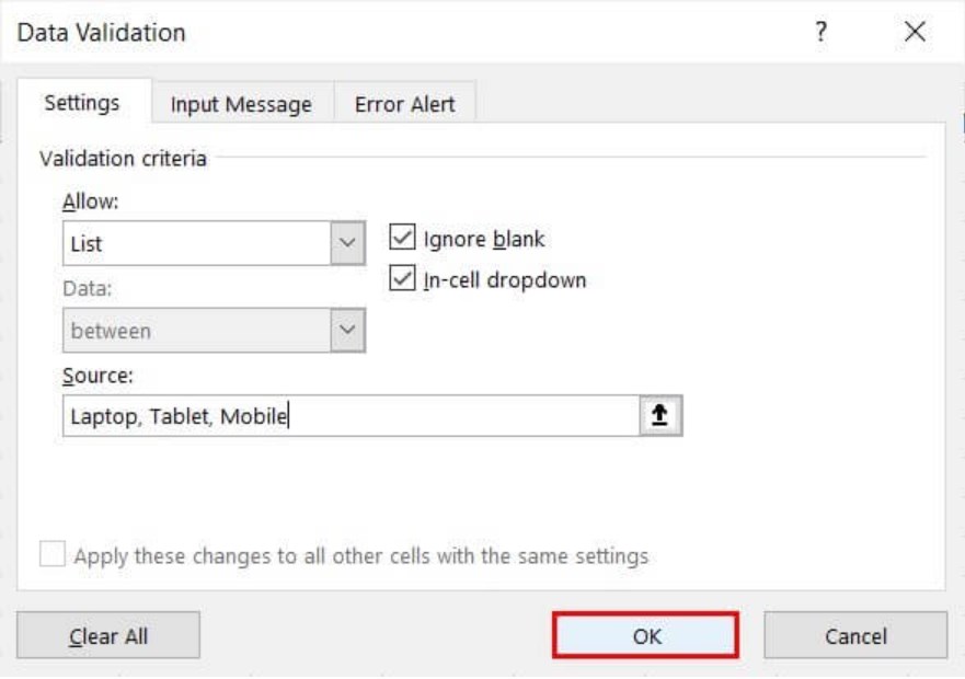
- Step 1: Select cell F5 which contains the word “laptop.” Delete this word.
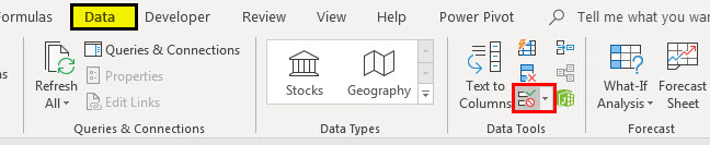
- Step 2: In the Data tab, go to the “data tools” section.
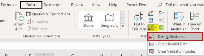
- Step 3: Select “data validation” from the drop-down list.
- Step 4: In the “data validation” dialog box, select “list” under “allow” criteria. In “source,” type “laptop, tablet, mobile” as these are the unique products. Click “Ok.”
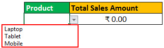
- Step 5: The drop-down list is created, as shown in the following image.
- Step 6: In the previous formula (under “step 1” of “example #1”), enter the reference of cell F5 in the “criteria” argument. Press the “Enter” key and the output appears (same as “step 2” of “example #1”).
With every change in the value of cell F5, the “total sales amount” updates automatically. The value in cell F5 is selected from the drop-down list.
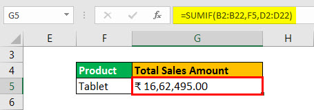
If “tablet” is selected, the tablet sales amount appears in cell G5.
#3–Text Criteria (Partial Match)
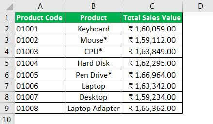
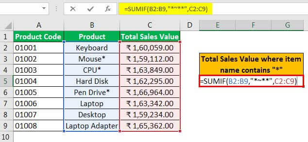
The following table shows the product-wise sales of an organization. The asterisk (*) indicates the items having high profit margins.
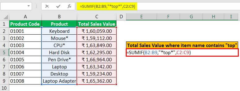
We want to sum the sales of the products which contain the word “top.”
We apply the formula shown in the following image.
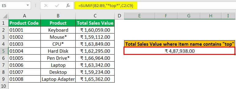
The output appears as shown in the succeeding image. It calculates the sum of the “laptop,” the “desktop,” and the “laptop adapter.”
#4–Wildcard Character
Working on example #3, we want to sum the sales of the products containing the asterisk.
The asterisk (*) is a wildcard character of Excel. To find this character, we use the escape character tilde (~).
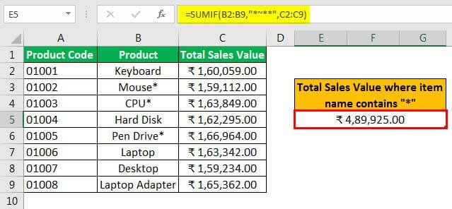
We apply the formula shown in the succeeding image.
The first and the last character of the criteria argument (*~**) is an asterisk. This suggests that the asterisk can be placed anywhere in the name of the product. It can either be the first character, the last character, or any character in-between.
Following the first asterisk is a tilde (~) sign with another asterisk (*). This implies that the formula should pick those products which contain the asterisk symbol.
The output of the formula is shown in the following image.
The Caution While Specifying Range
In the SUMIF formula, the “range” and the “sum_range” argument must be of the same size. In other words, the numbers of rows and columns of both ranges must be equal.
If the condition is satisfied, the formula begins summing with the first cell (top left) of the “sum_range.” It includes the same number of rows and columns as the “range.”
Note: This caution also applies to the SUMIFS function.
Frequently Asked Questions (FAQs)
1. How is SUMIF with multiple criteria used for two columns in Excel?
For every column, a SUMIF formula should be written. The multiple results are then added using the SUM function. The combined formula is given as follows:
“=SUM(SUMIF(range, criteria, sum_range),SUMIF(range, criteria, sum_range))”
Note: If there are more columns, more SUMIF formulae can be added to this combined formula.
2. How is SUMIF with multiple criteria used for an array in Excel?
The “range” and the “sum_range” arguments must always be entered as ranges. If an array (like 5,6,7,8) is entered in the SUMIF formula, it returns an error.
For example, the formula “=SUMIF(A1:A3,“sunflower”,B1:B3)” is correct. The formula “=SUMIF({“rose”,”sunflower”,”lotus”},“sunflower”,B1:B3)” is incorrect.
3. How is SUMIF used with two conditions in Excel?
The SUMIF with multiple criteria helps find the sum of numbers that satisfy either of the two given conditions. This is the OR logic and the formula is given as follows:
“=SUMIF(range,criteria1,sum_range)+SUMIF(range,criteria2,sum_range)”
The formula looks for numbers that satisfy either “criteria 1” or “criteria 2” and returns their combined sum.
- The SUMIF with multiple criteria sums the cell values based on the conditions provided.
- The SUMIF function works with a single criterion while the SUMIFS function works with multiple criteria.
- The criteria argument of the SUMIF function is based on dates, numbers, and text.
- The SUMIF function works with text criterion that is entered using a drop-down list.
- The various comparison operators and wildcard characters (* and ?) can be used in the criteria argument of the SUMIF function.
- The SUMIF function works with multiple criteria when used with the OR logic.
Recommended Articles
This has been a guide to SUMIF with multiple criteria in Excel. Here we provide step by step guide along with 4 example case studies. You may also look at these useful functions in Excel –