SUMIFS With Dates

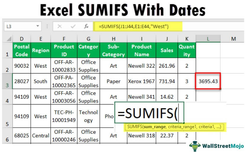
The SUMIFS function is used when there are more than one criteria; when fulfilled, the range of cells is summed. This function also supports dates as the criteria and the operators for the criterion.

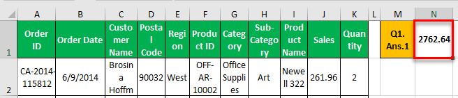
Suppose someone asks you, “What are the total sales for Office Supplies in the West Region? Here, we have two criteria: 1 – “Office Supplies” from “Category” and 2 – “West” from the “Region” column.

The actual formula will be =SUMIFS(J2:J51,G2:G51,” Office Supplies”,E2:E51,” West”)

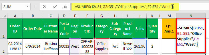
The answer is 2762.64.

• SUMIFS with Excel function helps users obtain the sum with criteria, including dates.
• The syntax of SUMIFS with dates is =SUMIFS( Sum range, Range for Date, Criteria Date, Range for Date 2, Criteria Date 2) where all the arguments are mandatory.
• SUM_range is the cell range used to evaluate based on specified criteria.
• Criteria_range1 and criteria1 denotes the range of cells specifying 1st criteria and the first criterion to be specified from criteria_range1, respectively.
• Similarly, criteria_range2 and criteria2 denotes the range of cells specifying 2nd criteria and the first criterion to be specified from criteria_range2, respectively.

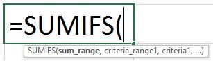
SYNTAX: =SUMIFS(sum_range, criteria_range1, criteria1, , ,…)

Arguments of Syntax:

• SUM_range: Sum_range is the range of cells you want to evaluate based on specified criteria.
• Criteria_range1: criteria_range1 is the range of cells from where you would like to specify 1st criteria.
• Criteria1: Criteria 1 is the first criterion that needs to be specified from criteria_range1.
• Criteria_range2: If you look at the syntax, criteria_range2 seems optional. The range of cells from which you would like to specify the second criteria.
• Criteria2: Criteria 2 is the second criterion that needs to be specified from criteria_range2.

We will learn how to use SUMIFS with the following example.

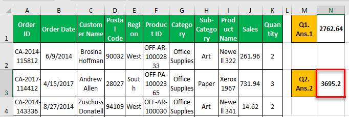
Question: What is the total sales value of the “West” region before 2017?

Solution: Apply formula =SUMIFS(J2:J51,E2:E51,” West,” B2:B51,” <1/1/2017″), and it will give you the total sales value of “Orders Date” before 1/1/2017 for the “West” region.

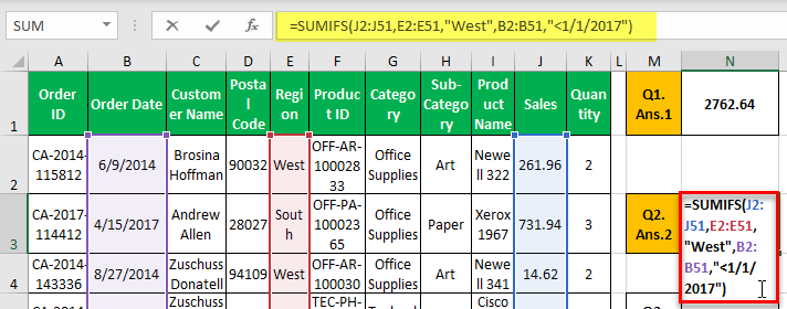
The answer is 3695.2.

Likewise, we can use SUMIFS with dates in Excel. For better understanding, we will use the same data with different years in the following examples.

Example #1

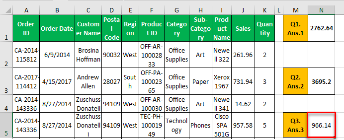
Question: What is the total sales value of “Phones” (Sub-Category) from the “West” region before 8/27/2017?

Solution: Here, you need to get sales based on three conditions: – “Sub-Category,” “Region,” and “Order Date.” Here you need to pass criteria_range3 and criteria3 as well.

Apply formula =SUMIFS(J2:J51,E2:E51,” West”,H2:H51,” Phones”,B2:B51,” < 8/27/2017″). It will give you the total sales value of “Phones” (Sub-Category) from the “West” region before 8/27/2017.

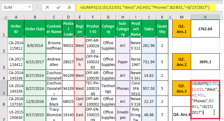
The answer is 966.14.

Example #2

Question: What is the total sales value of orders in 2017?

Solution: You can see that here you need to get the sales value of a given year. However, you do not have year fields in the data. Instead, you only have "Order Date," so you can pass two conditions, 1st – "Order Date" is greater than or equal to 1/1/2017, and 2nd condition – "Order Date "is less than or equal to 12/31/2017.

Here, you need to apply the following SUMIFS formula for dates.

=SUMIFS(J2:J51,B2:B51,”>=1/1/2017″,B2:B51,”<=12/31/2017″)

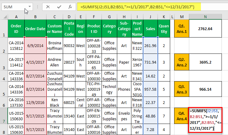
As you can see, we have also passed excel logical Operator “=”. Hence, this will include both dates.

The answer is 5796.2.

Example #3

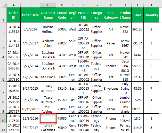
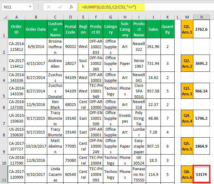
Question: Someone asks you to get the sales value for all those orders where we did not have a customer name who purchased our product.

Solution: You can see several orders where the customer name is blank.

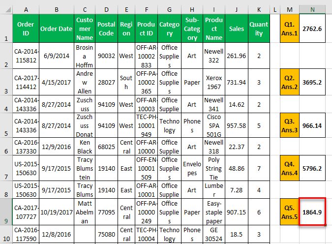
Here, you need to apply the following SUMIFS formula for dates =SUMIFS(J2:J51, C2:C51,”)

This formula will calculate only those cells with no value in the customer name field. If you pass “” (space in between the inverted comma), this will not give accurate results as space itself is considered a character.

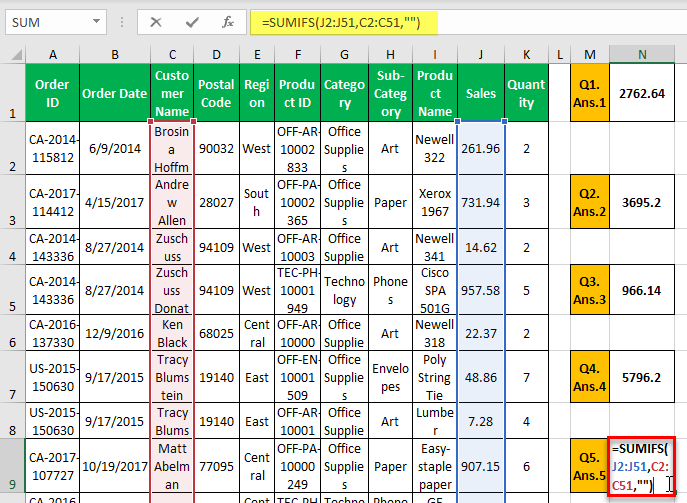
The answer is 1864.86.

• SUMIF is an useful function as sometimes, we don’t have to calculate the total of all data but some specific data.
• During such times, SUMIF is useful.
• Similarly, when dates are also a criteria, we can use SUMIFS with dates function.

This article is a guide to SUMIFS with Dates. Here, we will learn how to sum values between two date ranges in Excel, practical examples, and a downloadable Excel template. You may learn more about Excel from the following articles: -

• What is SUMIFS With Multiple Criteria?
• How to Sum Multiple Rows in Excel?
• SUM Shortcut in Excel
• SUMIF With VLOOKUP Explanation