Trunc in Excel

Last Updated :

21 Aug, 2024

Blog Author :

Edited by :

Reviewed by :

Table Of Contents

Trunc Function in Excel

The TRUNC is the Excel function used to trim decimal numbers to integers. It is one of the trigonometry and mathematical functions introduced in the 2007 version of Excel. The TRUNC function returns only the integer part by eliminating the fractional portion of a decimal number by specifying the required precision.

For example, TRUNC(5.8) will return 5.

Even though the INT function is also used for returning the integer part, it has a drawback. When the INT function in excel is used for negative numbers, it rounds the value to a lower number instead of the resulting integer. The present article explains the use of the TRUNC function in Excel with examples and formulas by covering the following topics.

Trunc Function in Excel

Explanation

The TRUNC function returns the trimmed value of a number based on the number of digits. It is a built-in function utilized as an Excel worksheet function. Moreover, it will be input as a formula into the cells of the Excel sheet.

Syntax

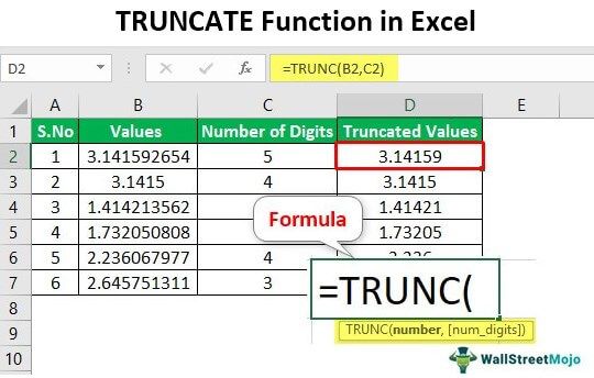
Parameters Required: The parameters used by the TRUNC function are identified as number and num_digits.
Number: It is the mandatory parameter that a user wants to truncate the digits of the fractional part.
num_digits: The optional parameter specifies the number of digits to be truncated after decimal numbers. The default value of this parameter is 0 if no value is given.
Returns: This function results in a numeric number omitting the fractional part.

This function works in all Excel versions, including 2007, 2010, 2013, 2016, and office 365.

If the value is given to the parameter of num_digits:

Value is equal to zero. The function returns the rounded value.
The value is more than zero. It indicates the number of digits to be truncated and presented on the right side of the decimal.
The value is less than zero. It shows the number of digits to be truncated and displayed on the left side of the decimal.

How to Use the Truncate Function in Excel? (Example)

Example #1 - Basic Usage of TRUNC Function

This example best illustrates the basic applications of the truncated function.

The steps to use the TRUNC function in Excel are as follows:

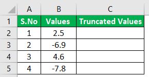
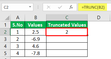
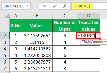
In the first step, consider the following data shown in the figure.
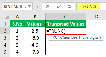
Place the cursor into the appropriate cell to enter the TRUNC function in Excel.
Enter the Excel truncate formula as shown in the figure.
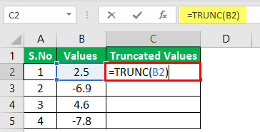
Select the cell address of the number that wants to be truncated.
In this, no cell address is given for the num_digits parameter, and it takes the default value of zero. Press the "Enter" key to see the result.
Apply the formula to the remaining cells by dragging through the mouse.
Observe the results shown as mentioned below screenshot.

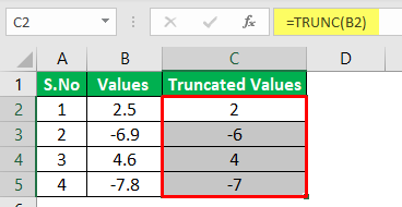
Only the left part of the decimal results since the default value is zero.

Example #2 - Applying TRUNC Function on a Set of Decimal Numbers

This example best illustrates the basic applications of the truncated function on the set of decimal numbers.

Step 1: In the first step, consider the following data shown in the figure.

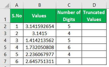
This example will truncate the number of digits after the decimal point is considered.

Step 2: Place the cursor into the appropriate cell.

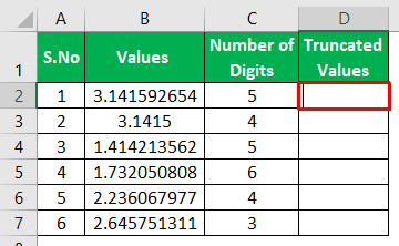
Step 3: Enter the TRUNCATE Excel function as shown in the figure.

Step 4: Select the cell address of the number that wants to be truncated and the number of digits.

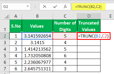
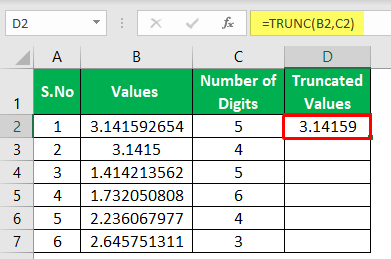
This cell address is given for values and num_digits parameters, taking the value mentioned in the column. Press the "Enter" key to see the result, as shown below.

Step 5: Apply the formula to the remaining cells by dragging them through the mouse.

Step 6: Observe the results displayed as mentioned below screenshot.

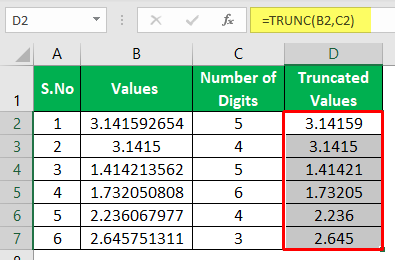
In this, the right part of a decimal number results from the value given in the column of several digits. A number of digits 5 indicates a decimal number is truncated to 5 digits after the decimal point.

Example #3 - To Extract Date from Date and Time

Step 1: In the first step, consider the following data shown in the figure.

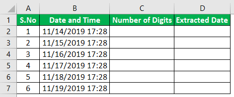
In this example, the number of digits for extracting the date is regarded as zero.

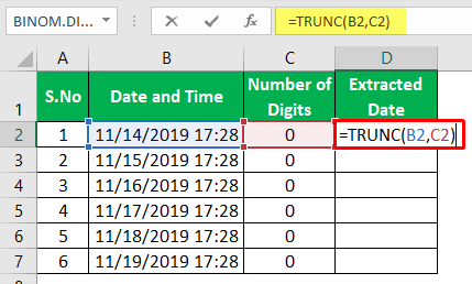
Step 2: Place the cursor into the appropriate "Extracted Date" cell to enter the TRUNC function in Excel.

Step 3: Enter the TRUNCATE Excel function as shown in the figure.

In this, cell address is given for date and time and num_digits parameter as zero, as mentioned in the column.

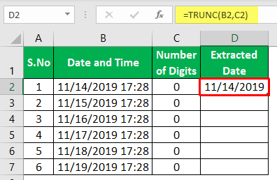
Step 4: Press the "Enter" key to see the result below.

Step 5: Apply the excel formula to the remaining cells by dragging through the mouse.

Step 6: Observe the results displayed as mentioned below screenshot.

As shown in the figure, only the date value is extracted from the date and time using the TRUNCATE function in Excel. If we do not give a number, it takes the default value of zero to the result date.

Application

The TRUNC function has a lot of applications in Excel:

For example, this Excel function is useful in financial analysis to trim the values to preferred precision levels.
It is used in mining the time and date values from the date.
Truncating a decimal number to the nearest integer number
It is used when there is no need for the grounding of a number.

Things to Remember

The INT and TRUNCATE Excel functions are identical since they result in integer values. But, these are different when they are used with negative, For example, INT(-5.3) returns -6 since it is a lesser value, but TRUNC (-5.3) returns -5, only removing the fractional value.
When num_digits is negative, it returns the truncated value as zero.