SWITCH Excel Function

The SWITCH Excel Function is a comparison and referencing function that compares and matches a referred cell to a group of cells and returns the result based on the first match found.

The Excel Switch function is an inbuilt function in Excel so that we can insert it from the “Function Library”, or enter it directly in the worksheet.

For example, we will replace the cell A1 value with a new value. Enter the formula =SWITCH(A1,“IND”,“INDIA”) in cell B1 and press “Enter”, as shown below.

The output is shown above, i.e., the selected cell value, IND, is replaced with the new value INDIA.

• The SWITCH Excel Function helps users replace a cell value with a new value with the syntax =SWITCH( target cell, value 1, result 1….) based on the result’s published value.
• The function is introduced and available in Excel 2016 on Windows and MAC, but not in earlier versions of Excel.
• We can take 126 pairs of values and results into the Excel SWITCH function.
• We have the default value in the SWITCH function, which is not in the IF function.
• The function is different from the VLOOKUP, but we can use it along with the VLOOKUP function.

The syntax of the SWITCH Excel formula is,

The arguments of the SWITCH Excel formula are,

• expression – The value or expression to match which is against. It is a mandatory argument.
• value1, result1 – The first value and result pair. It is a mandatory argument.
• value2, result2 – The second value and result pair. It is an optional argument.
• default – The default value to use when no match is found.

We can use the SWITCH Excel Function in 2 ways, namely,

1. Access from the Excel ribbon.
2. Enter in the worksheet manually.

Method #1 – Access from the Excel ribbon

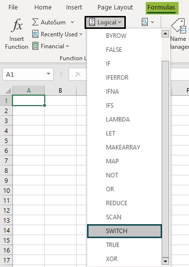
Choose an empty cell - select the “Formulas” tab - go to the “Function Library” group - click the “Logical” option drop-down - select the “SWITCH” function, as shown below.

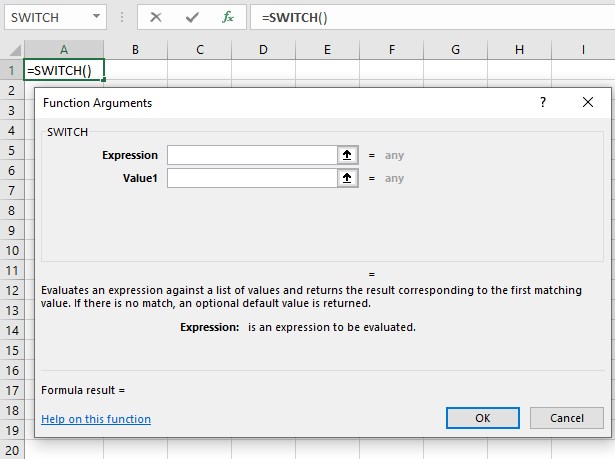
The “Function Arguments” window appears. Enter the arguments in the “Expression” and the “Value1” fields, and click “OK” as shown below.

Method #2 – Enter in the worksheet manually

1. Select an empty cell for the output.
2. Type =SWITCH( in the selected cell.
3. Enter the arguments as cell values or cell references.
4. Close the brackets and press the “Enter” key.

This article must help understand SWITCH Excel function with its formula and examples. You can download the template here to use it instantly.

We will consider an example of the Switch formula and the explanation of the same.

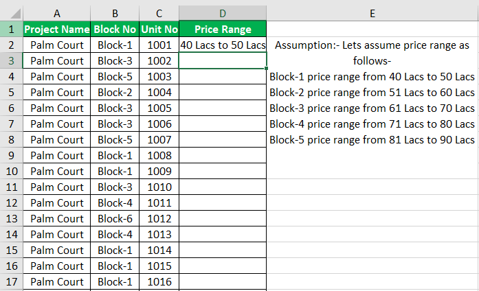
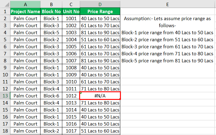
In the table given above, we can note the following data,

1. One of the projects is the name “Palm Court.”
2. Different blocks that are available in the project.
3. Other unit numbers are available in the project for their respective blocks.
4. It is the “Price Range” that we are supposed to determine as per the assumption taken.
5. Cell D1, or cell 1 in the Price Range column, has a formula inserted that is explained below.

#Switch Formula

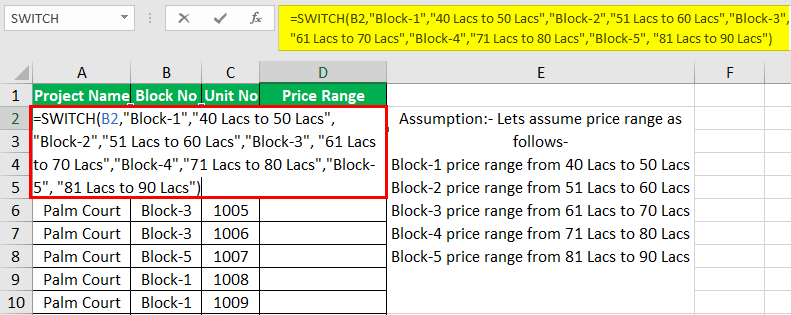
The formula inserted is shown below.

Let us look at the SWITCH formula to obtain the value of cell 2, i.e., cell D2, in the “Price Range” column:

• The SWITCH function is available in Excel 2016.
• In this example, we have to take the block cell as the expression, as the assumptions of prices are based on block numbers.
• Value1 and Result 1 – We have mentioned that if an expression matches value 1, then take result 1 or go to condition 2.
• Value 2 and Result 2 – If condition 1 is not satisfied, then the expression comes to condition 2 to check whether it will get the match to obtain result 2. This step will continue until the expression matches the value.
• If the expression does not match any value in the conditions, it will give a #NA error as output, as shown below in cell D13.

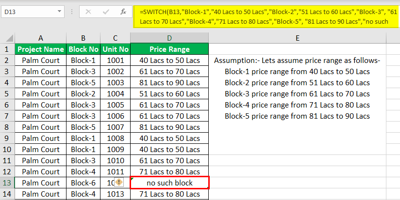
To mention some statements for the cells that are showing #NA, we can give a string within inverted commas as below:

If we evaluate the above problem using the IFs function, we need to have an Excel nested IF for “True” or “False,” which is not a LOOKUP function. When it is “True”, it gives out one result, and for “False,” it gives other results.

A few differences between the SWITCH and the IF functions are as follows:

• The SWITCH function does not allow us to use logical operators in excel like greater than (>) / less than (<) to match the cases where there will not be an exact match.
• The expression will appear only once in the Excel SWITCH function, but in the IF’s function, the expression needs to be repeated.
• The SWITCH function’s length is less than the IF’s function, making it easier to read and create as it allows us to test more than one condition.
• It is more like a CHOOSE function in Excel. It has an expression that is a lookup value. We would match it to value 1 and value 2 and get the result value. Unlike the IF function, we have the default value in the SWITCH function.

• The function will return the #NA error if we do not mention any default condition, and if any condition does not get the match.
• However, as a negative, we cannot use logical operators such as >, <, or = in the expression. It simply matches the values in its list to the expression and cannot test if a value is larger or smaller.

This article is a guide to SWITCH Excel Function. Here we use Switch to replace cell values, instead of IF(), CHOOSE, VLOOKUP, examples & downloadable template. You may also look at these useful functions in Excel: -

• Calculate P-Value in Excel
• ISNA Function in Excel
• VALUE Function in Excel
• TRANSPOSE Function in Excel